1
2
3
4
A B C D E F G H I J K L M N O P Q R S
12 Chapter model 12/12/2018
9/12/2022 16:03
This worksheet contains a model to analyze Allied’s new expansion project, Project S. Models for analyzing
replacement decisions, risk analysis, and an abandonment option discussed within the text are provided on
Chapter 12. Cash Flow Estimation and Risk Analysis
Page 1
ΔNOWC = Additional net operating working
capital
7
8
9
10
11
12
13
16
17
18
19
30
31
32
33
36
37
38
41
42
A B C D E F G H I J K L M N O P Q R S
EXPANSION PROJECT ANALYSIS (Section 12-2)
Table 12.1 Cash Flow Estimation and Analysis for Expansion Project S
0 1 2 3 4 Cash flows based on Straight Line Depr’n 0 1 2 3 4
Investment Outlays at Time = 0 Investment Outlays at Time = 0
Unit sales 2,720 2,640 2,515 2,430 Unit sales 2,720 2,640 2,515 2,430
Sales price $2.00 $2.00 $2.00 $2.00 Sales price $2.00 $2.00 $2.00 $2.00
Variable cost per unit $1.0196 $1.0404 $1.0457 $1.1973 Variable cost per unit $1.020 $1.040 $1.046 $1.197
Terminal Cash Flows at Time = 4 Terminal Cash Flows at Time = 4
Salvage value (taxed as ordinary income) 50 Salvage value (taxed as ordinary income) 50
13 13
After-tax salvage value 37 After-tax salvage value 37
Alternative depreciation Straight line 0 2 3 4
Cost: $1,200 Rate 25% 25% 25% 25%
Bonus
Depreciation
NPV $78.82
ΔNOWC = Recovery of net operating
ΔNOWC = Recovery of net operating
Formulas
Straight line
=NPV(D40,F35:I35)+E35
$16.56
All dollars (expect for sales and costs per unit values) and unit sales are shown in thousands. Data are
taken from Chapter 12.
Life (Time = 1 – 4)
Life (Time = 1 – 4)
Tax on salvage value = 0.25 × (SV − BV of
equipment at t = 4)
Tax on salvage value = 0.25 x (SV – BV of
equipment at t = 4)
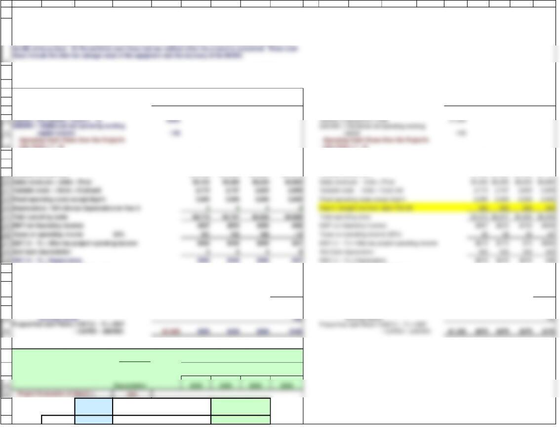
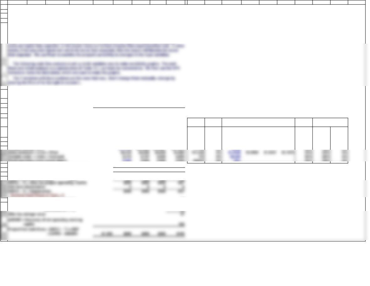
The main model, on this tab, evaluates Project S. Table 12.1 divides the project’s cash flows into three
components. (1) The initial investments that are required at t = 0. These include capital expenditures and
changes in net operating working capital (ΔNOWC). (2) The operating cash flows the company receives over
Page 2
43
A B C D E F G H I J K L M N O P Q R S
IRR 14.489%
=IRR(E35:I35)
10.700%
Page 3
46
47
48
50
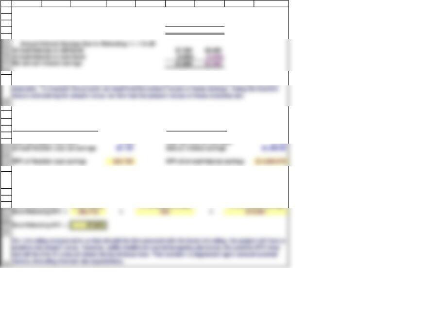
Based on the 10% WACC, the project’s NPV is $78.82. Since the NPV is positive and both the IRR and MIRR
exceed the WACC, we tentatively conclude that the project should be accepted. Note, though, that no risk
analysis has been conducted. It is possible that Allied’s managers, after appraising the project’s risk, might
1. Under the new tax legislation, 100% of the cost of certain new and used business assets may be
immediately expensed if placed into service after September 27, 2017 and before January 1, 2023.
For assets placed into service after January 1, 2023 but before January 1, 2027, only 80% of the
asset’s cost may be immediately expensed. Immediate expensing is eliminated after January 1,
rate.
2. If the firm owned assets that would be used for the project but would be sold if the project is
3. If this project would reduce sales and cash flows from one of the firm’s other divisions, then
cash flows shown on row 29.
4. If the firm had previously incurred costs associated with this project, but those costs could not
10.349%
12 Chapter model
Table 12.2 Replacement Project R
0 1 2 3 4
Sales revenues $2,500 $2,500 $2,500 $2,500
Operating costs except depreciation 1,140 1,140 1,140 1,140 Costs except depreciation: Old $1,140 $1,140 $1,140 $1,140
Depreciation 100 100 100 100 New 400 400 400 400
Total operating costs $1,240 $1,240 $1,240 $1,240 ∆$740 $740 $740 $740
∆$100 $100 $100 $100
New machine invest. after 100% bonus depr.
-$2,000
After-tax salvage value, old machine 400
CAPEX, after taxes -$1,600
Sales revenues $2,500 $2,500 $2,500 $2,500
Costs except depreciation 400 400 400 400
Depreciation 0 0 0 0
Total operating costs $400 $400 $400 $400
EBIT (or Operating income) $2,100 $2,100 $2,100 $2,100
Taxes 25% 525 525 525 525
EBIT(1 − T) = After-tax operating income $1,575 $1,575 $1,575 $1,575
Add back depreciation 0 0 0 0
Part III. Incremental Cash Flows and Evaluation
-$1,600 $530 $530 $530 $530
Project Evaluation @ WACC = 10%
NPV = $80.03
Part II. Free Cash Flows After Replacement:
New Machine ( ΔNOWC = 0)
Incremental CFs = CF After — CF Before
9/12/2022 16:03
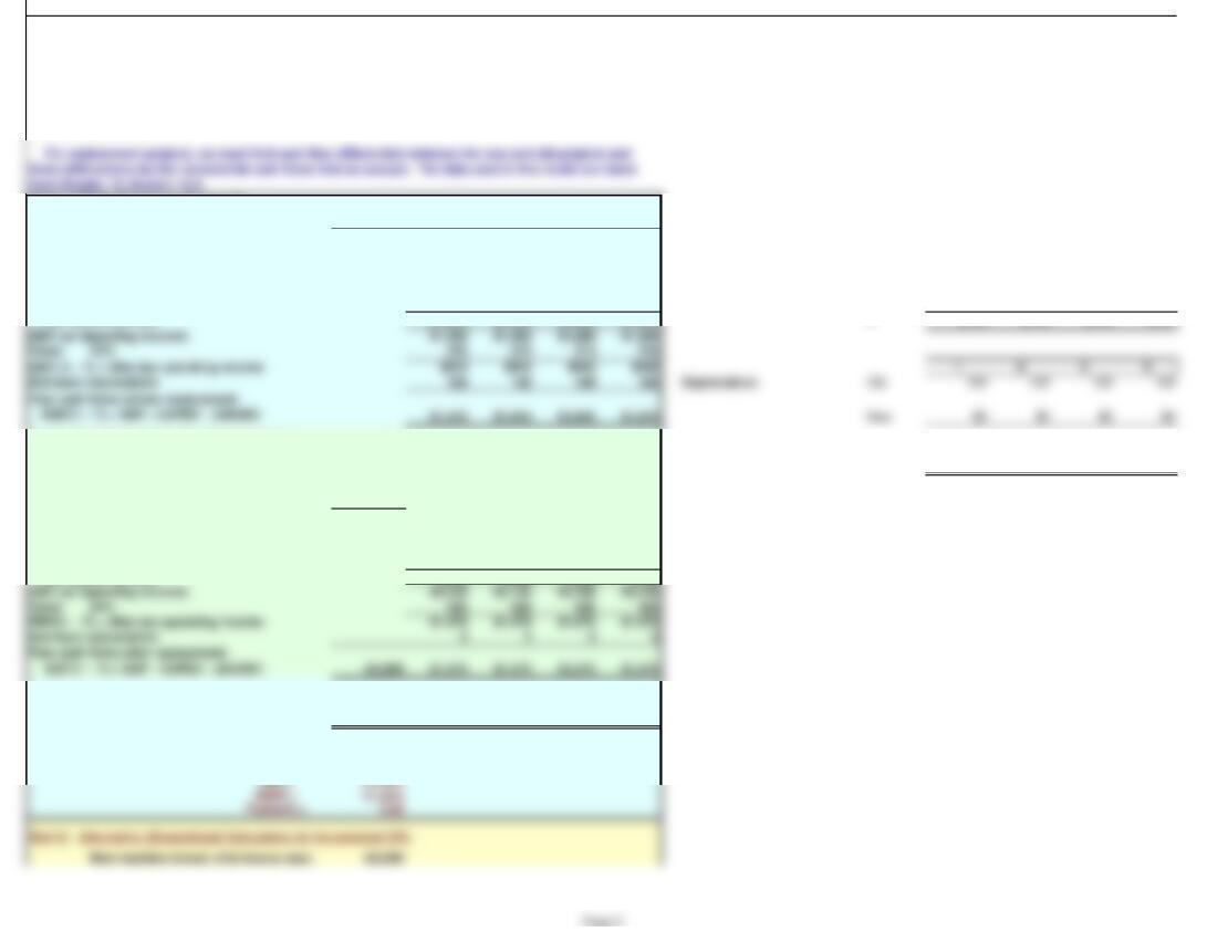
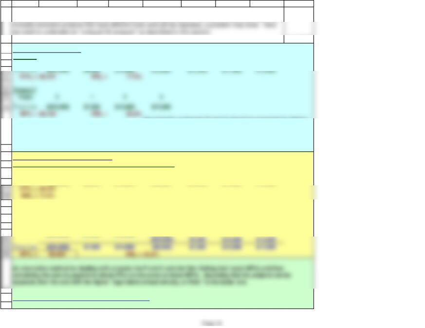
REPLACEMENT ANALYSIS (Section 12-3)
This model analyzes decisions related to replacing assets that are currently being used with more efficient
assets. While the mechanics of the analysis are somewhat different from that used for a new project, the
concepts are identical.
these differentials are the incremental cash flows that we analyze. The data used in this model are taken
from Chapter 12, Section 12-3.
Part I. Free Cash Flows Before Replacement:
Old Machine (CAPEX and ΔNOWC = 0)
12/12/2018
Taxes 25% 315 315 315 315
EBIT (1 − T) = After-tax operating income $945 $945 $945 $945 1 2 3 4
Add back depreciation 100 100 100 100 Depreciation: Old 100 100 100 100
46
47
48
49
55
A B C D E F G H I J K L M N O P Q R
Salvage value, old machine 400
Net cost of new machine -$1,600
Cost savings = Old — New $740 $740 $740 $740
A-T savings = Cost savings × (1 — Tax rate) 555 555 555 555
Page 6
1
2
EBIT(1 − T) = After-tax project operating income $500 $400 $300 –$37
EBIT(1 − T) + Depreciation $500 $400 $300 –$37
3
4
9
10
11
12
13
14
15
16
17
18
19
22
23
24
25
26
31
A B C D E F G H I J K L M N O P Q R S T
12 Chapter model 12/12/2018
Table 12.1 Cash Flow Estimation and Analysis for Expansion Project S
0 1 2 3 4
Investment Outlays at Time = 0
CAPEX = Equipment = Cost (1 − T) -$900
-100
Variable Case Worst Best Base
Equipment 0% $900 25% -25% 0%
Unit sales 2,720 2,640 2,515 2,430 WC 0% $100 25% -25% 0%
Sales price $2.00 $2.00 $2.00 $2.00 Units 0% 2,720 2,640 2,515 2,430 -25% 25% 0%
Variable cost per unit $1.0196 $1.0404 $1.0457 $1.1973 Price 0% $2.00 -25% 25% 0%
Fixed operating costs except depr’n 2,000 2,000 2,000 2,000 WACC 0% 10% 25% -25% 0%
Depreciation: 100% Bonus Depreciation in Year 0 0 0 0 0
Total operating costs $4,773 $4,747 $4,630 $4,909
EBIT (or Operating income) $667 $533 $400 –$49
Taxes on Operating income 25% 167 133 100 -12
Salvage value (taxed as ordinary income) 50
Setup for scenarios. The zeros in column L are changed manually, which changes values of the
cash flows to get changing NPVs. Note that 0% is the Base Case, +25% is good for Units and
Price, whilce -25% is good for the other variables. The reverse is true for the Worst Case. For
scenarios, change all the variables. You can copy and paste the %’s in columns Q, R, and S into
column L to create the scenarios. End by pasting the Base Case zeros back in column L.
9/12/2022 16:03
RISK ANALYSIS IN CAPITAL BUDGETING (Section 12-4)
SENSITIVITY ANALYSIS
Cash flows under this case
Tax on salvage value = 0.4 × (SV − BV of
equipment at t = 4)
Risk in capital budgeting essentially means the probability that the actual outcome will be much worse
than the expected outcome. For example, if there were a high probability that the $78.82 expected NPV as
calculated previously will turn out to be quite negative, then the project would be classified as relatively
risky. The reason for a worse-than-expected outcome is, typically, that sales are lower than expected,
ΔNOWC = Additional net operating working
capital needed
Operating Cash Flows Over the Project’s
Life (Time = 1 – 4)
Page 7
37
38
39
40
43
44
45
46
47
48
49
50
51
52
53
54
57
58
59
60
61
62
63
64
65
66
74
75
76
77
78
79
80
81
82
83
84
85
86
A B C D E F G H I J K L M N O P Q R S T
Project Evaluation @ WACC = 10.00%
Bonus
Depreciation
NPV $78.82
IRR 14.489%
Data tables used to make sensitivity graph:
Deviation Sales Price Deviation Unit Sales Deviation VC/Unit
from Base $78.82 from Base $78.82 from Base $78.82
Best 25% $3,155.25 Best 25% $1,513.83 Worst 25% -$1,562.60
Deviation Fixed Costs Deviation Equipment Deviation WACC
from Base $78.82 from Base $78.82 from Base $78.82
Worst 25% -$1,109.88 Worst 25% -$146.18 Worst 25% $33.62
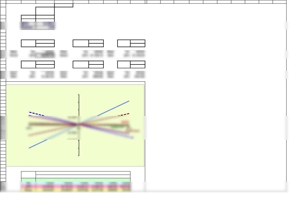
Figure 12.1 Sensitivity Graph for Project S
Deviation
from Base Sales Price VC/Unit Units Sold Fixed Costs Equipment WACC
25% $3,155.25 –$1,562.60 $1,513.83 -$1,109.88 -$146.18 $33.62
NPV with Variables at Different Deviations from Base
-$4,000
-$3,000
-$2,000
$2,000
$3,000
$4,000
NPV
Percentage Deviation from Base
Price
Units
Page 8
41
42
91
92
94
95
96
We see from the graph and the tables that NPV is quite sensitive to changes in the sales price, fairly
sensitive to changes in variable costs, a bit less sensitive to units sold and fixed costs, but not very
sensitive to changes in the equipment cost or the WACC.
2. If the sales price is set 25% above its expected $2 price and all other variables are set at
their expected values, then the NPV would be +$3,155.25. If the price is set 25% below its
3. Note that the best- and worst-case NPVs are different from those in the next section, which
shows scenario analysis. In scenario analysis, all the variables are 25% above or below their
1. When all of the inputs are set at their base case levels, their deviations from base are all zero,
and the NPV is $78.82. So, the vertical axis intercept is at $78.82.
Page 9
-$6,049.17
0 $78.82
$9,354.43
99
100
101
102
103
104
105
106
107
108
109
115
116
117
118
119
120
121
122
123
131
132
133
134
135
138
139
140
A B C D E F G H I J K L M N O P Q R S T
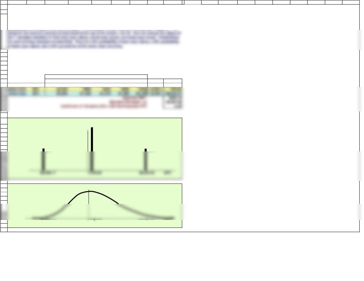
Figure 12.2 Scenario Analysis for Project S
Cash Flows Under Alternative ScenariosPredicted Cash Flow for Each Year
Prob: 0 1 2 3 4 WACC NPV
Best Case 25% -$750 $3,300 $3,131 $2,920 $2,637 7.50% $9,354.43
Discrete Probabilities
Continuous Probabilities
NPV
Probability Density
-$6,049.17
0 $78.82
$9,354.43
SCENARIO ANALYSIS
Scenario analysis extends risk analysis in two ways: (1) It allows us to change more than one variable at a
time, hence to see the combined effects of changes in several variables, and (2) It allows us to bring in the
Probability
25%
25%
50%
Page 10
141
142
149
150
151
152
159
160
161
162
A B C D E F G H I J K L M N O P Q R S T
Prob.
NPV @
12.5%
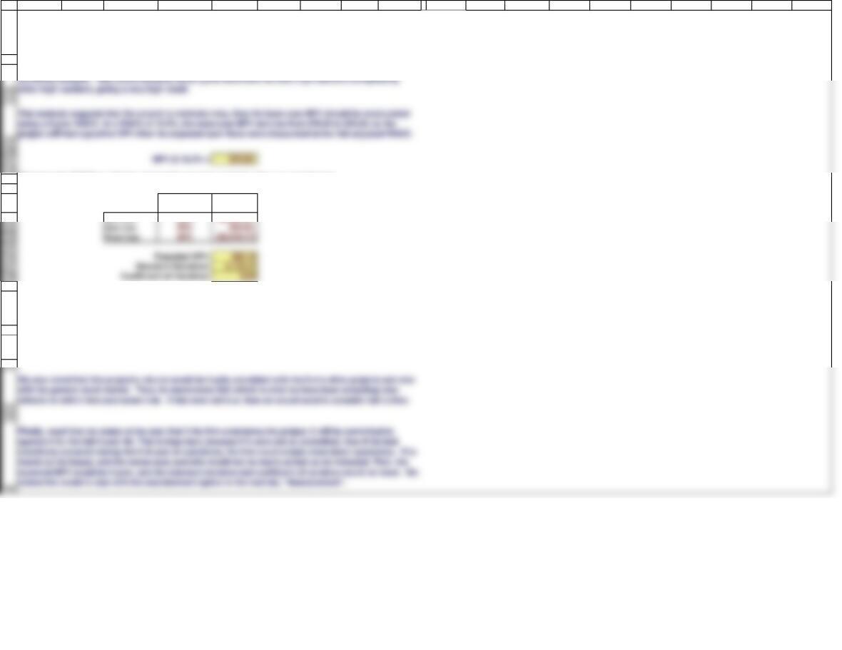
Best Case 25% $8,354.51
If the bad conditions occur, this will hurt but not bankrupt the firm–this is just one project for a large
company.
The scenario analysis suggests that the project would be profitable ($865,730), but it is quite risky. There is
a 25% probability that the project would result in a loss of $6,049,170. There is also a 25% probability that
it could produce an NPV of $9,354,430. The standard deviation is high, at $5,502,550, and the coefficient of
variation is aso high, 6.36.
Note that the expected NPV in the scenario analysis is much higher than the expected NPV in the
Changing the WACC would also change the scenario analysis. Here are new figures:
Based on the analysis to this point, the project looks risky but acceptable. There is a good chance that it
will produce a positive NPV, but there is also a chance that the NPV could be dramatically higher or lower.
Page 11
1
2
3
4
5
6
7
8
9
10
11
19
20
21
22
23
24
31
32
33
34
46
A B C D E F G H I J
12 Chapter model 12/12/2018
REAL OPTIONS: The Abandonment Option (Section 12-7)
We use Project S to illustrate the abandonment option. Up to this point we have assumed
that the project would be operated for its full 4-year life. Now we assume that the company
can close the project down after it has gone into operation if it so chooses.
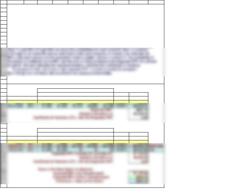
We show below decision trees for three scenarios under the “No Abandonment” and “Can
Abandon” cases. Cash flows are taken from the Scenario Analysis model, where they were
calculated. In the column for Time 0, we show that the firm must invest between $750 and $1,250.
Table 12.3 Decision Tree For Abandonment Option (Dollars in Thousands)
Situation 1. No Abandonment
Predicted Cash Flow for Each Year
Prob. 0 1 2 3 4 WACC NPV
Best Case 25% –$750 $3,300 $3,131 $2,920 $2,637 7.50% $9,354.43
Situation 2. Can Abandon
Predicted Cash Flow for Each Year
Prob. 0 1 2 3 4 WACC NPV
Best Case 25% –$750 $3,300 $3,131 $2,920 $2,637 7.50% $9,354.43
9/12/2022 16:03
Page 12
Then, in cells B24 through B26, we show the probabilities for each scenario. Next, in columns
C through G, we show the annual cash flows under each scenario. In column I we calculate the
NPV under each scenario at the scenarios’ costs of capital, shown in column H. The probability of
the branch is multiplied by its NPV, and the sum of these products is the Expected NPV. It is shown
in cell I27. We next calculate the standard deviation, and then the coefficient of variation.
but if things turn out badly, this would hurt the company rather badly.
47
48
49
50
A B C D E F G H I J
The possiblity of abandonment increases the expected NPV because some negative CFs will
not occur. The standard deviation also declines. Both of these changes cause the CV to
decline. The project’s CV ends up above 2.0, which is the average CV for the firm’s projects,
which in turn suggests that it is appropriate to evaluate the project using WACC = 12.5%.
Page 13
Finally, note that the difference between the expected NPV with and without abandonment
represents the value of the option to abandon.
It often turns out that without abandonment, the bad case outcome is so bad that it causes the
expected NPV to be negative, hence causes the project to look unacceptable. However, when
abandonment possibilities are factored in, the worse-case outcome is not nearly as bad, and the
expected NPV becomes positive. Clearly, abandonment option possibilities must be considered
to obtain valid assessments for different projects.
1
2
3
4
5
6
7
8
9
10
15
16
17
24
Immediate tax savings on old flotation cost expense 2,400 600
Extra interest paid on old issue (600) (450)
Interest earned on short-term investment 300 225
18
19
20
A B C D E F G H I
REFUNDING OPERATIONS (WEB APPENDIX 12B)
12/12/2018
Table 12B.1 Bond Refunding Analysis
Input Data (in thousands of dollars)
Existing bond issue $60,000 New bond issue $60,000
Original flotation cost $3,000 New flotation cost $2,650
Maturity of original debt 25 New bond maturity 20
Cash flow schedule
Before-tax After-tax
Investment Outlay
Call premium on the old bond ($6,000) ($4,500)
Flotation costs on new issue (2,650) (2,650)
This example examines the issue of replacing existing debt with newly issued debt. At its core, this issue
raises two important questions. First, “Is it profitable to call an outstanding issue and replace it with a new
issue?” Second, even if refunding now is profitable, “Would the firm’s expected value be further increased if
the refunding were postponed until a later date?”
Page 14
Years since old debt issue 5New cost of debt 9%
Call premium (%) 10%
Original coupon rate 12% Tax rate 25%
After-tax cost of new debt 6.75% Short-term interest rate 6%
26
27
28
29
30
After-tax cost of new debt 6.75% After-tax cost of new debt 6.75%
Annual flotation cost tax savings $3.125 Annual interest savings $1,350.00
NPV of flotation cost savings $33.759 NPV of annual interest savings $14,584.079
52
53
35
37
38
39
40
41
46
47
48
49
50
A B C D E F G H I
Annual Flotation Cost Tax Effects: t = 1 to 20
Annual tax savings from new issue flotation costs $132.500 $33.125
Annual lost tax savings from old issue flotation costs (120.000) (30.000)
Annual net flotation cost tax savings
$12.500 $3.125
Calculating the annual flotation cost tax effects and the annual interest savings
Annual Flotation Cost Tax Effects Annual Interest Savings
Maturity of the new bond 20 Maturity of the new bond 20
Bond Refunding NPV =
Initial Outlay
+ +
Since the annual flotation cost tax effects and interest savings occur for the next 20 years, they represent
Hence, the net present value of this bond refunding project will be the sum of the initial outlay and the
present values of the annual flotation cost tax effects and interest savings.
PV of flotation costs
PV of interest savings
Page 15
34
Annual Interest Savings Due to Refunding: t = 1 to 20
Annual interest on old bond $7,200 $5,400
Annual interest on new bond (5,400) (4,050)
Net annual interest savings $1,800 $1,350
1
2
3
4
11
12
13
14
15
16
19
20
21
22
23
27
28
29
A B C D E F G H I
12/12/2018
Part I. Traditional Analysis WACC = 12%
Project C
Years 0 1 2 3 4 5 6
Part II. Replacement Chain Adjustment WACC = 12%
Project C (Identical to the analysis in Part I. Just repeated here.)
Years 0 1 2 3 4 5 6
Time Line:
($40,000) $8,000 $14,000 $13,000 $12,000 $11,000 $10,000
Project F: Replacement Chain modification to create common life.
0 1 2 3 4 5 6
($20,000) $7,000 $13,000 $12,000
Part III. Equivalent Annual Annuity (EAA) Method
1. Find the NPV of each first cycle investment as was done in Part I above.
Mutually Exclusive and Repeatable Projects with Unequal Lives: If we are choosing between two
Here it looks as though Project C should be accepted, but that is
incorrect, because, as demonstrated below, Project F can be
selected, then repeated at the end of its life, and the result is a
higher “extended life” NPV.
($40,000) $8,000 $14,000 $13,000 $12,000 $11,000 $10,000
30
31
32
33
37
Project C Project F
PV: $6,491 $5,155
Inputs:
2. Find the annual annuity payment that is equivalent to each project’s NPV, i.e., has the same present value. We
know the projects’ NPVs and lives, and we know the WACC, so we can find the resulting payment, which is the EAA.
Page 17
1
2
3
4
5
6
7
8
15
16
17
18
19
20
21
22
23
32
A B C D E F G H I J
REAL OPTIONS 12/12/2018
Table 12F.1 Illustration of a Timing Option (Dollars in Millions)
Situation 1. Proceed Immediately: Invest Now
Predicted Cash Flow for Each Year
Situation 2. Delay Decision: Invest Only If Conditions Are Good
Predicted Cash Flow for Each Year
Prob. 0 1 2 3 4 5 WACC NPV @ t = 1
Good 50% -5.0 2.5 2.5 2.5 2.5 10.00% $2.92
Bad but
irrelevant
50% 0000010.00% 0.00
Expected NPV $1.462
Standard Deviation (s)$1.462
Coefficient of Variation (CV) = Std Dev/Expected NPV 1.00
Below, we show examples of two different real options: a timing option and a growth option. Williams
Inc. is considering a project that requires an initial investment of $5 million at the beginning of 2015 (or
t = 0). The project will generate positive cash flows at the end of each of the next four years (t = 1, 2, 3,
and 4). However, the size of each annual cash flow will depend on what happens to market conditions
in the future.
Having the ability to delay the investment increases the expected NPV and reduces risk (because the
CV declines from 2.38 to 1). This occurs because the firm can gather more information to decide
Page 18
Good 50% -5.0 2.5 2.5 2.5 2.5 10.00% $2.92
Standard Deviation (s)$2.060
Coefficient of Variation (CV) = Std Dev/Expected NPV 2.38
35
36
38
39
40
Good 50% -3.00 1.50 1.50 1.50 12.00% $0.603
62
41
42
43
44
45
49
50
51
52
53
54
63
64
A B C D E F G H I J
Table 12F.2 Analysis of a Growth Option (Dollars in Millions)
Situation 1. No Growth Option
Predicted Cash Flow for Each Year
Prob. 0 1 2 3 WACC NPV
Situation 2. Project with Growth Option
Predicted Cash Flow for Each Year
Prob. 0 1 2 3 WACC NPV
Good 50% -3.00 1.50 1.50 1.50
-10.00 20.00
Finally, note that the difference between the expected NPV with and without the timing option
represents the value of the timing option.
We can illustrate the growth option with a distribution center in mainland China being considered by
the Crum Corporation. An investment of $3 million would be required at t = 0. Under good conditions
New investment
Page 19