
CHAPTER 12
Aggregate Demand II:
Applying the IS–LM Model
Notes to the Instructor
1929. They may also want to draw parallels with the bursting of the so–called “Internet bubble”
and the subsequent retreat of the stock market in 2000–2001. The lessons that the Great
Depression teaches about the importance of financial and credit markets are also timely given
the problems of U.S. banks and savings institutions in the early 1990s, the Asian financial crisis
of the late 1990s, and the worldwide financial crisis of 2008-2009. (For instructors who wish to
pursue the subject of the stock market, Chapter 17 of the Instructor’s Resources contains a series
of chapter supplements on asset pricing, including discussions of stock market efficiency.)
Use of the Web Site
The Chapter 12 model can be used to derive aggregate demand curves by making use of the fact
that increases in the price level and decreases in the nominal money stock have identical effects
(this is a useful lesson to drive home anyway). Thus, one can find {M, Y} pairs for which the
money and goods markets are in equilibrium and then convert this to the corresponding {P, Y}
pairs.
Use of the Dismal Scientist Web Site

268 | CHAPTER 12 Aggregate Demand II: Applying the IS–LM Model
Chapter Supplements
This chapter includes the following supplements:
12-1 Do High Deficits Cause High Interest Rates?
12-3 Credit Rationing and the Great Depression
12-5 Proportional Income Taxes and the IS Curve
12-6 Additional Readings
Lecture Notes | 269
Lecture Notes
12–1 Explaining Fluctuations with the IS–LM Model
We have now developed the basic IS–LM model of the economy and are in a position to use it to
try to explain the behavior of the economy in the short run. Output can vary in the IS–LM model
whenever exogenous shocks to the economy cause shifts in either the IS or the LM curve.
How Fiscal Policy Shifts the IS Curve and Changes the Short–
Run Equilibrium
Let us first consider fiscal–policy shocks. Suppose that we start in equilibrium and that
government spending is increased by ∆G. Then the IS curve shifts to the right. The increased
spending increases income and, through the multiplier effects from the circular flow, also
increases consumption; income increases further. [Recall that the rightward shift of the IS curve
How Monetary Policy Shifts the LM Curve and Changes the
Short–Run Equilibrium
Now consider the effects of an increase in the money supply (an expansionary monetary policy).
This shifts the LM curve out. The increased money supply causes interest rates to fall in order to
bring the demand for money in line with the new higher supply. This fall in interest rates
encourages investment, leading ultimately to an increase in GDP. Thus, interest rates are lower
and GDP is higher. The linkage from a change in the money supply to GDP is known as the
monetary transmission mechanism.
The Interaction Between Monetary and Fiscal Policy
The policy changes discussed above took the form of an exogenous change in one policy,
holding all other exogenous variables constant. In reality, monetary and fiscal policy do not exist
in isolation from each other. The Federal Reserve and the fiscal authorities both pursue policy
goals that may or may not be compatible. We consider the details and problems of policy–
making in Chapter 18. Here we note simply that the ultimate effects of a fiscal–policy change
depend upon how the monetary authorities react to that change.
Shocks in the IS–LM Model
The IS and LM curves shift whenever they are hit by exogenous shocks. We have already
discussed how changes in fiscal policy shift the IS curve and how changes in monetary policy
shift the LM curve. The IS curve also shifts if other components of planned spending change. For
example, the “animal spirits” of businesspeople shift the IS curve. Similarly, changes in
consumer confidence alter consumption behavior and cause the IS curve to shift. Shocks to the
!
Supplement 12-1,
“Do High Deficits
Cause High
Interest Rates?”
!
Figure 12-3
!
Supplement 12–2,
“Macroeconometric
Models”
270 | CHAPTER 12 Aggregate Demand II: Applying the IS–LM Model
financial side of the economy cause the LM curve to shift. In particular, anything that causes an
exogenous increase in money demand implies an inward shift of the LM curve.
Case Study: The U.S. Recession of 2001
The U.S. economy slowed sharply in 2001, with unemployment rising and output growth
stalling. Three major shocks can help understand the onset of this economic recession. First, the
stock–market boom of the 1990s ended abruptly in the spring of 2000 as optimism about new
information technology waned. The decline in the stock market lowered the wealth of
households and, in turn, lowered consumer spending. Also, the dimmed outlook for new
technologies led to a pullback in business investment. These effects can be interpreted as a shift
to the left in the IS curve. Second, the September 11 terrorist attacks on New York and
Washington led to a further decline in the stock market—which, at the time, was the largest one–
What Is the Fed’s Policy Instrument—the Money Supply or the
Interest Rate?
The analysis in this chapter assumes that the Fed influences the economy by controlling the
money supply, but the Fed’s short–term policy instrument is an interest rate target (the federal
funds rate). These are not inconsistent. To control the federal funds rate (the rate banks charge
one another for overnight loans), the Fed conducts open–market operations. These open–market
operations change the money supply, shifting the LM curve and thus changing the interest rate.
12–2 IS–LM as a Theory of Aggregate Demand
From the IS–LM Model to the Aggregate Demand Curve
We now consider how the IS–LM model can also be viewed as a theory of aggregate demand.
We defined the IS and LM curves in terms of equilibrium in the goods and money markets,
respectively. Aggregate demand summarizes equilibrium in both of these markets.
Thus we find that the aggregate demand curve is downward sloping; high values of the price
!
Figure 12-6
Lecture Notes | 271
The IS–LM Model in the Short Run and Long Run
We can also analyze the transition to the long run in the IS–LM model. If the economy is not at
full employment, then the price level adjusts. In terms of the AD–AS diagram, the economy
moves along the AD curve. In terms of the IS–LM diagram, the LM curve shifts. Thus we can see
that the process of adjustment to equilibrium has subtle economic forces lying behind it. If, for
example, we start in recession, then over time prices fall. This increases the real money supply,
pushing down interest rates and encouraging investment. This increase in investment, in turn,
leads to higher spending and higher GDP.
As another example, suppose that, starting in long–run equilibrium at the natural rate of
output, we increase government spending. In the short run, with the price level fixed, this leads
12–3 The Great Depression
In the 1930s, the United States and other economies experienced a severe depression. The desire
to explain this phenomenon was Keynes’s principal motivation for his new approach to
economics. The magnitude of the economic upheaval and the accompanying human misery, in
turn, fascinate economists and lead them to study the Great Depression to avoid any recurrence
of such an event. The data for the Great Depression years are set out in Table 12-1. Economists
have suggested a number of explanations for these data, each of which may contain part of the
truth.
The Spending Hypothesis: Shocks to the IS Curve
The IS–LM model teaches that an inward shift in the IS curve reduces income and interest rates.
Since nominal interest rates fell during the Depression, negative shocks to the IS curve are one
possible explanation. This is the spending hypothesis. Significant falls occurred in both
consumption and investment spending between 1929 and 1933. Consumption may have fallen
The Money Hypothesis: A Shock to the LM Curve
A particularly striking feature of the Depression–era data is the substantial fall in the money
supply (over 25 percent between 1929 and 1933). A monetary contraction shows up in the IS–
LM model as an inward shift of the LM curve, which would reduce output. There are two
problems with this money hypothesis, however. The first is that prices also fell substantially over
The Money Hypothesis Again: The Effects of Falling Prices Another aspect of
the money hypothesis is that even if both money and prices fell so that real money balances
changed little and the LM curve was hardly affected, the deflation itself might have played a
!
Figure 12-7
!
Table 12-1
!
Supplement 12–3,
“Credit Rationing
and the Great
272 | CHAPTER 12 Aggregate Demand II: Applying the IS–LM Model
major role in the Depression. The basic IS–LM model suggests that falling prices increase output
because falling prices increase real money balances for any given money supply. Falling prices
might also increase output because of the Pigou effect: Decreases in the price level increase the
real value of wealth, increasing consumption and shifting the IS curve out.
Other arguments, however, suggest that deflation might decrease output. Consider first the
effect of an unexpected fall in the price level. As explained in Chapter 5, this represents a
redistribution, in real terms, from debtors to creditors; a given nominal debt becomes larger in
real terms. Now suppose that creditors and debtors also differ in terms of their marginal
propensities to consume. In particular, it is reasonable to think that debtors have higher
propensities to consume than do creditors. Then the redistribution from debtors to creditors
reduces aggregate spending, shifting the IS curve in. This is known as the debt–deflation theory.
In an IS–LM diagram with the nominal interest rate on the vertical axis and income on the
horizontal axis, the position of the IS curve depends upon the expected inflation rate. Higher
expected inflation lowers the real interest rate, increases investment, and shifts the IS curve to
the right, thereby increasing output and raising the nominal interest rate. Conversely, lower
expected inflation (or higher expected deflation) raises the real interest rate, reduces investment,
and shifts the IS curve to the left, reducing output and lowering the nominal interest rate. .
Could the Depression Happen Again?
After the major stock market fall of October 1987, some commentators worried about whether
this might presage a severe decline in economic activity, just as the 1929 stock market crash did.
While economists cannot be completely confident that such a severe depression will never recur,
our greater understanding of the macroeconomy today does give modern policymakers a
significant advantage over their 1930s counterparts. Above all, the Fed is likely to avoid
Case Study: The Financial Crisis and the Great Recession of
2008 and 2009
During 2008, the U.S. economy experienced a financial crisis and economic downturn that to
some observers mirrored events from the 1930s. The crisis began with a boom in the housing
market a few years earlier, the result of low interest rates that made buying a home more
affordable. Increased use of securitization in the mortgage market further fueled the housing
boom by making it easier for subprime borrowers to obtain credit. These borrowers had a higher
risk of default that may not have been fully appreciated by the purchasers of mortgage–backed
securities (banks and insurance companies). The high level of house prices proved unsustainable
!Figure 12-8
!Table 12-2
Lecture Notes | 273
and prices fell by 30 percent from 2006–2009. This decline had several repercussions that
intensified what was a moderate–to–severe house–price correction into a full–blown crisis.
First, mortgage defaults and home foreclosures increased sharply, in large part due to loose
mortgage–lending standards that had permitted little or no money down on home purchases. As
prices fell, these homeowners were “under water,” and many decided to stop paying on their
mortgages. Sales of foreclosed properties further depressed house prices. Second, numerous
financial institutions suffered heavy losses on the mortgage–backed securities that they owned.
As a result, banks cut back on lending to other banks out of fear and distrust that they might not
be repaid. Third, companies that rely on the financial system for funds to run their business
found it difficult to obtain short–term loans. Concern about the profitability of these companies
led to sharp swings in their stock prices. Finally, gyrations in stock prices, in turn, led to a sharp
decline in consumer confidence and resulted in a huge drop in consumer spending.
Government responded strongly to the crisis. The Fed lowered its target for the federal
funds rate from 5.25 percent in September 2007 to approximately zero in December 2008.
Congress appropriated $700 billion for the Treasury to use to stabilize the financial system by
The Liquidity Trap (also known as the Zero Lower Bound) Interest rates
reached levels close to zero in the United States during the 1930s and, more recently, during late
2008, when the Fed lowered its target for the federal funds rate to a range of zero to 0.25 percent
and kept it there for several years. Economists refer to this situation as a liquidity trap. Because
nominal interest rates cannot fall below zero, an expansion in the money supply would not be
able to lower nominal interest rates and therefore might not be able to affect spending. The
economy could become “trapped” at a low level of aggregate demand, output, and income. But
since spending directly depends on real interest rates rather than nominal rates, a higher rate of
inflation could push real interest rates below zero and stimulate spending. This is the reason why
some economists argue for targeting a rate of inflation that is above zero—say, around 4 percent
per year. Such an inflation target would give the central bank the ability to lower the real interest

12-4 Conclusion
The IS–LM model with fixed prices is still an incomplete model of the economy in the short run.
!Supplement 12–4,
275
12–1 Do High Deficits Cause High Interest Rates?
The IS–LM model of Chapter 12 predicts that expansionary fiscal policy—that is, increases in government
spending or decreases in taxes, both of which imply increases in the deficit—leads to high interest rates.
Increases in the deficit increase the demand for goods and services and thus shift the IS curve to the right.
The associated increase in income increases the demand for money, and so interest rates must rise to keep
the money market in equilibrium. In the long run, the effect is even stronger: Increases in the price level
cause the LM curve to shift back to the left, resulting in still higher interest rates. This can be seen
equivalently in the classical model of Chapter 3; that model shows how increases in the deficit decrease
national saving and so increase interest rates.
Increases in interest rates in turn imply reduced investment—crowding out—in both the short run and
the long run. Economists worry, therefore, that high deficits imply low levels of investment, leading
ultimately to a lower capital stock and so lower living standards. It is, therefore, important to see if this
prediction that high deficits lead to high interest rates is supported by the data.1
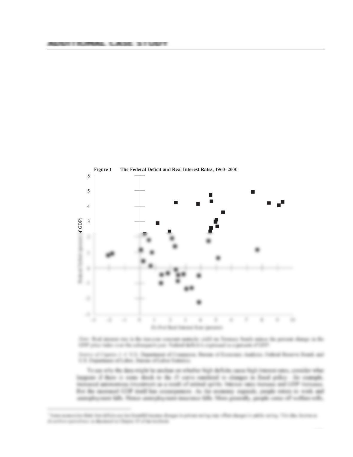
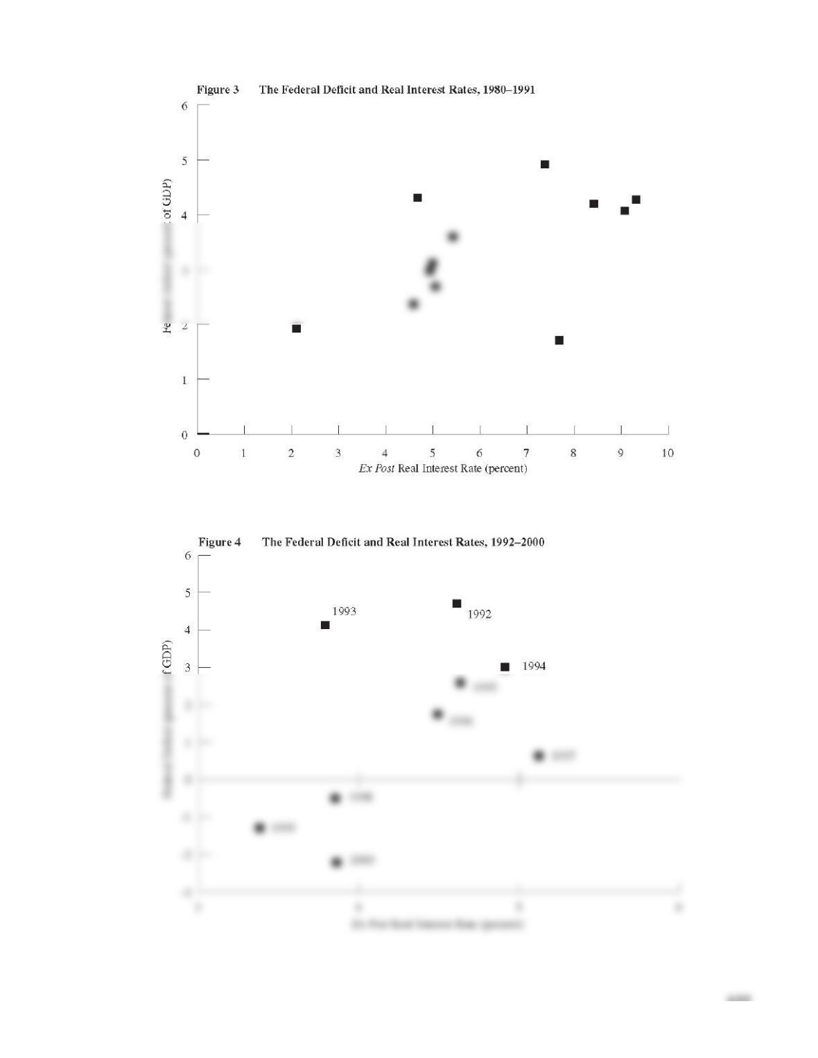
Like many empirical questions in economics, this one is difficult to answer unequivocally. Figure 1
shows a scatterplot of the real government deficit and the ex post real interest rate between 1960 and 2000.
While there is some evidence of a positive association, it is not strong.
and transfers such as Medicaid fall. Further, increased GDP means that the government takes in more in
tax revenues. The presence of these automatic stabilizers results in a decrease in the deficit. (Automatic
stabilizers are discussed in more detail in Chapter 18 of the textbook.) In the data, we would observe
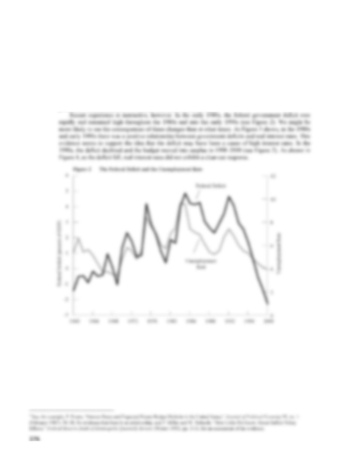
interest rates rising and the deficit falling, although there was no direct causal link between the two. Figure
2 illustrates this relationship between the unemployment rate and the federal deficit.
Exactly the opposite would occur given an LM shock (the result, for example, of a change in money
demand or money supply). If the LM curve shifts out, we observe interest rates falling and the deficit
falling, but again with no causal link. The data are thus likely to be substantially contaminated by these
sorts of effects, since shocks other than changes in the deficit are likely to swamp the effects of exogenous
changes in the deficit. Overall, economists have not yet managed categorically to establish either the
presence or the absence of a link between deficits and interest rates.2
277
Although interest rates rose at first as the deficit declined, they fell sharply during the last three years
of the decade. Thus, disentangling the effect of deficits on real interest rates remains a difficult task.
ADDITIONAL CASE STUDY
12–2 Macroeconometric Models
To estimate the magnitude of the effects of policy changes, economists sometimes use large–scale
macroeconometric models of the economy. These models use statistical and econometric techniques to
analyze the economy. On the basis of existing data, it is possible to obtain estimates of the magnitude of
key parameters, such as the marginal propensity to consume. The model with these estimated parameters
Fair’s model is more complicated partly because he considers more disaggregated data (and so has
three different consumption functions, for example), partly because he considers labor–market variables
and asset–market variables that are not included in a simple IS–LM model, and partly because he considers
price adjustment.
Models such as Fair’s were initially developed in the 1950s, and at one time the refinement of these
criticism. Lucas pointed out that these models might not be good for evaluating different economic
policies because agents will change their behavior in response to changed policies. Thus, according to
Lucas, it does not make sense to suppose that a behavioral equation estimated under one set of policies
will be unchanged when policies are changed.
Fair, not surprisingly, is a strong advocate of the usefulness of large–scale models of the economy,
ADDITIONAL CASE STUDY
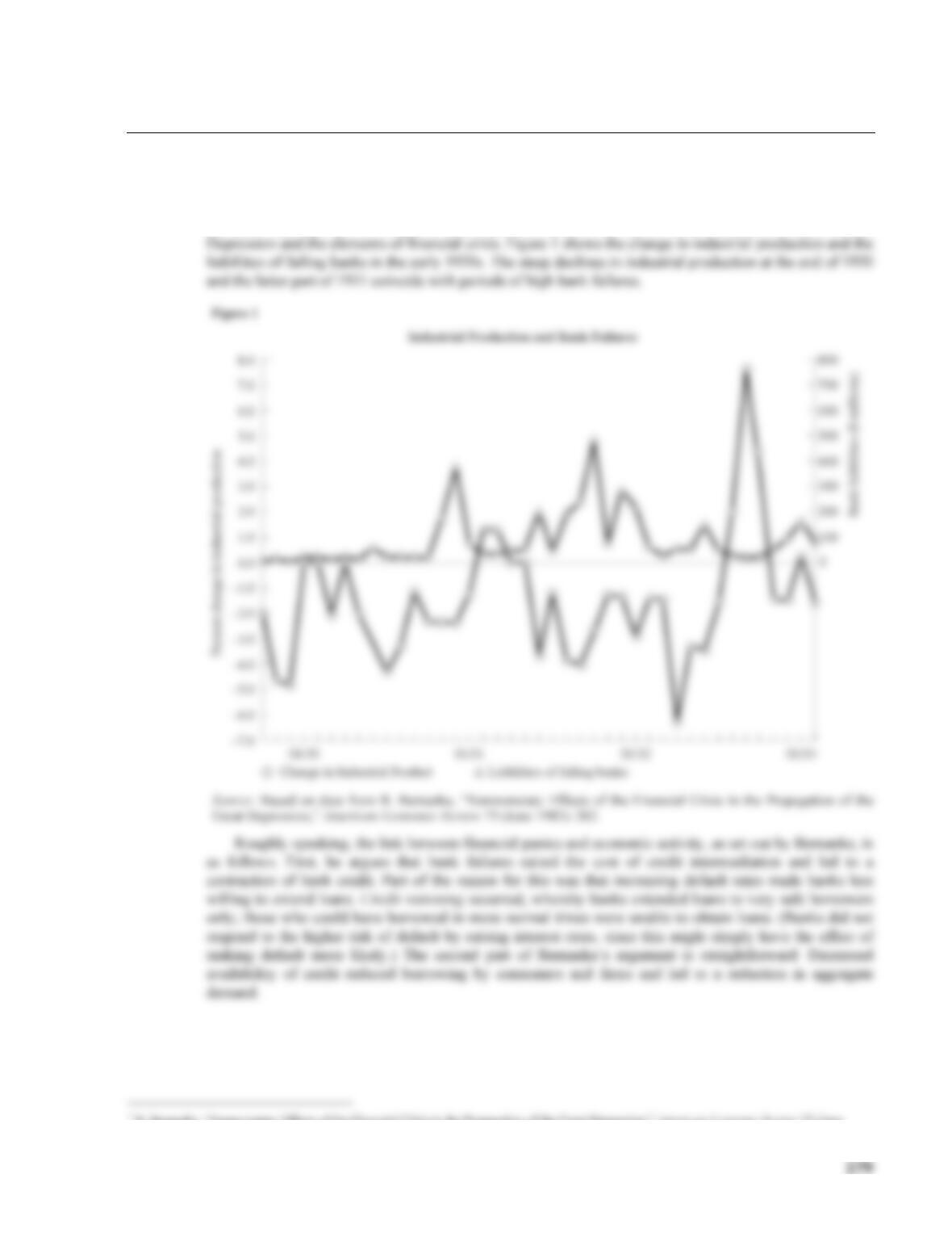
12–3 Credit Rationing and the Great Depression
Economist and former Fed Chair Ben Bernanke has made a strong case that failures in credit markets were
an important aspect of the Great Depression.1 As noted in Chapter 12 of the textbook, this is an element of
the spending hypothesis. Bernanke documents the connection between the decline in output in the
1983): 257–76.
LECTURE SUPPLEMENT
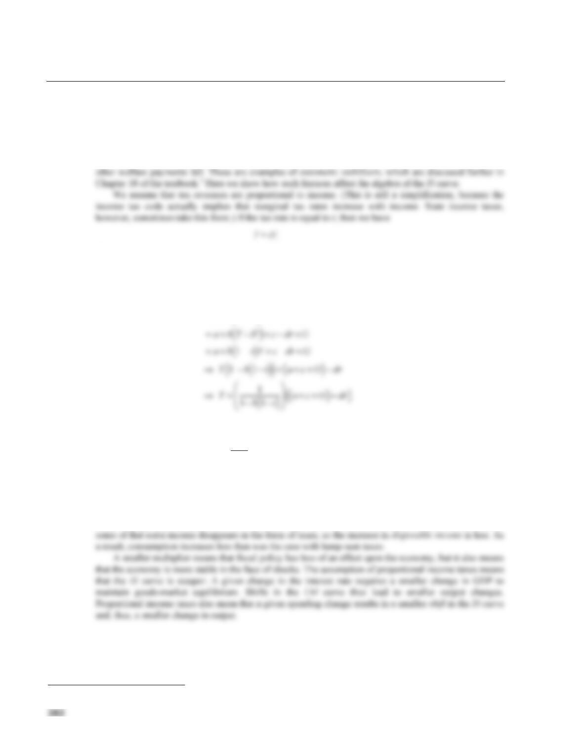
12-4 The Simple Algebra of the IS–LM Model and Aggregate Demand
Curve
The IS Curve
To analyze the mathematics of the IS curve, let us suppose that
C(Y – T) = a + b(Y – T)
explains how much Y changes for a given change in G, holding r fixed. It thus tells us how far to the right
the IS curve shifts for a given increase in G. (See Supplement 12-5, “Proportional Income Taxes and the IS
Curve” for details of how proportional taxes affect the IS curve.)
The LM Curve
Let us suppose a simple linear expression for money demand:
L(r, Y) = eY – fr
⇒ M/P = eY – fr.
The Aggregate Demand Curve
Substituting for r from the LM curve into the IS curve yields
Y=1
1−b
a+c+G−bT
( )
−d elf
( )
Y−1 / f
( )
M/P
( )
( )
⇒Y1+de /f
+M/P
The Effectiveness of Monetary and Fiscal Policy
Around the 1960s, the biggest debate in macroeconomics was probably the one centering on the relative
efficacy of fiscal and monetary policies. Some economists implied that d was small by arguing that
investment was not very responsive to the interest rate. The aggregate demand equation then implies that
monetary policy cannot have a big effect on output. When investment does not respond to interest rate
changes, a crucial link in the monetary transmission mechanism breaks down. We can interpret this in
terms of the IS–LM diagram: When d is small, the IS curve is steep, so shifts in the LM curve result in
large changes in interest rates and small changes in GDP.
Other economists, known as monetarists, believed that money demand was not very responsive to the
LECTURE SUPPLEMENT
12-5 Proportional Income Taxes and the IS Curve
The textbook makes the simplifying assumption that the level of (net) tax revenue, T, is independent of the
level of GDP. In reality, we expect that T is likely to increase as Y increases. There are two reasons for
this. First, income taxes are important in the United States. Income taxes imply that the government
collects more tax revenue when income is higher. Second, transfer payments go down as income
increases—when the economy is booming, more people are employed, so unemployment insurance and
The remainder of our analysis is as before:
C = a + b(Y – T)
I = c – dr.
Substituting into the goods–market equilibrium condition (Y = C + I + G), we get
Y=a+b Y –T
( )
+c–dr +G
Our earlier equation for the IS curve was
Y=1
1−b
⎛
⎝
⎜⎞
⎠
⎟a+c+G−bT
( )
−dr
( )
.
Comparing the two, we see that the new IS curve no longer contains a bT term. This is because the level of
tax revenue, T, is no longer an exogenous variable in the model. More important, we see that the multiplier
term, which was previously 1/(1 – b), is now 1/(1 – b(1 – t)). Proportional income taxes reduce the value
of the multiplier. This can be understood in terms of the circular flow of income. Suppose, as considered
in the text, government purchases are increased. This increases GDP and so increases income. But now
1 See also the discussion of the Great Depression in Chapter 12 of the textbook and Supplement 12–1, “Do High Deficits Cause High Interest Rates?”

LECTURE SUPPLEMENT
12-6 Additional Readings
The Spring 1993 edition of the Journal of Economic Perspectives contains a symposium on the Great
Depression, with articles by Christina Romer, Robert Margo, Charles Calomaris, and Peter Temin.
Economists have, of course, written a great deal on the Depression; a good place to start is Peter Temin’s
book, Lessons From the Great Depression (Cambridge, Mass.: MIT Press, 1989).
For some interpretations of the most recent recession, see G. Perry and C. Schultze, “Was This
Recession Different? Are They All Different?” Brookings Papers on Economic Activity 1 (1993): 145–