Economics Chapter 12 Discuss the challenges and costs of reducing

Chapter 12

Unemployment and Inflation

◼ Learning Objectives

I. Goals of Part 4

A. How macroeconomic policy works and how it can best be used

1. Unemployment and inflation (this chapter)

II. Goals of Chapter 12

A. Describe the Phillips curve relationship between unemployment and inflation (Sec. 12.1)

B. Discuss whether the Phillips curve offers a ‘menu’ of inflation-unemployment combinations

III. Notes to Eighth Edition Users

A. We add a discussion of the problems that arise if inflation is too low

Chapter 12 Unemployment and Inflation 273

◼ Teaching Notes

I. Unemployment and Inflation: Is There a Trade-off? (Sec. 12.1)

A. Many people think there is a trade-off between inflation and unemployment

1. The idea originated in 1958 when A.W. Phillips showed a negative relationship between

unemployment and nominal wage growth in Britain

inconsistent with the Phillips curve

B. The expectations-augmented Phillips curve

1. Friedman and Phelps: The cyclical unemployment rate (the difference between actual and

2. How does this work in the extended classical model?

Analytical Problem 3 looks at similar analysis in a Keynesian model.

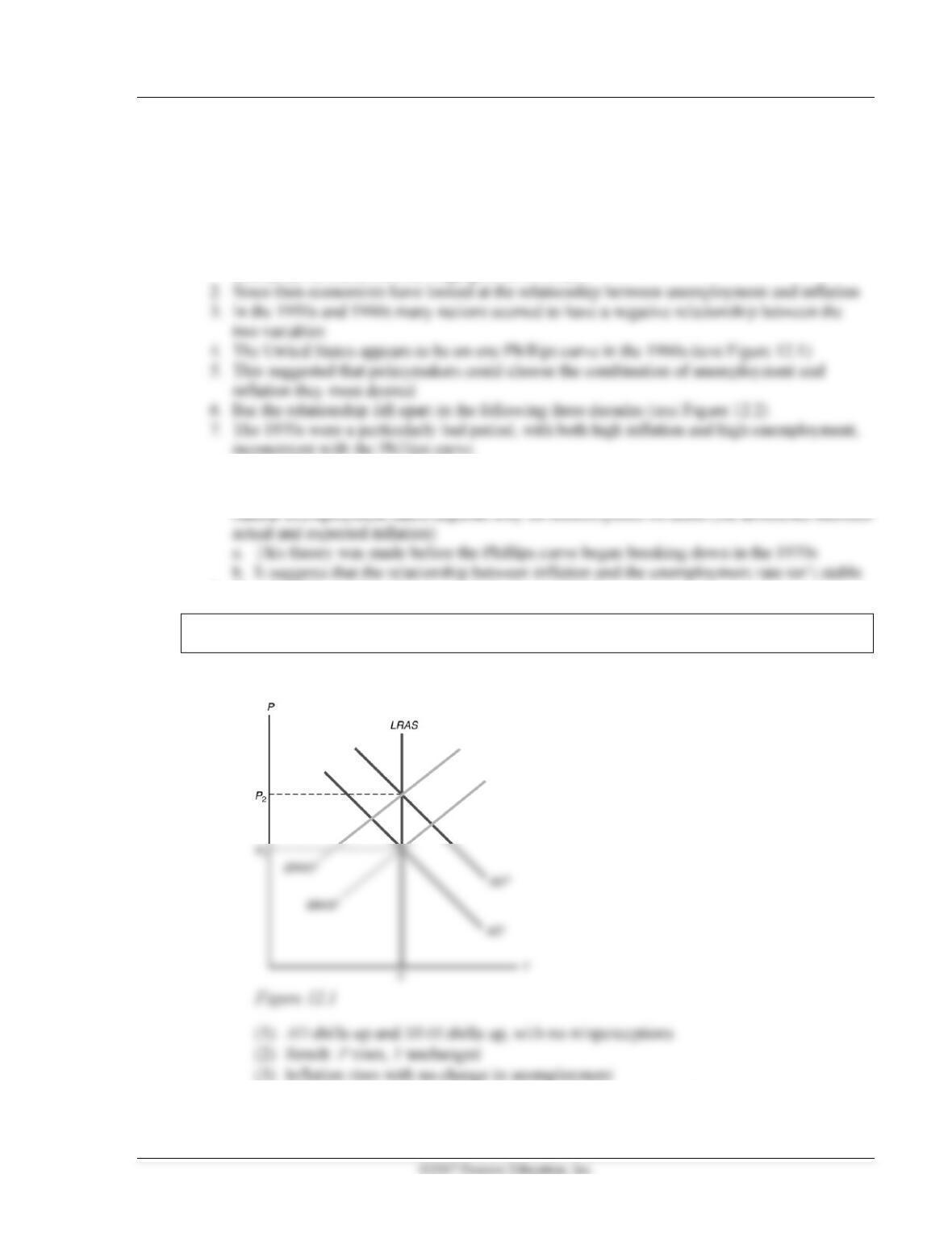
a. First case: anticipated increase in money supply (Figure 12.1; like text Figure 12.3)

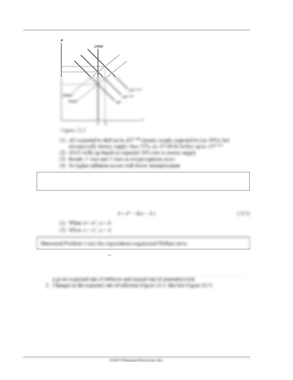
b. Second case: unanticipated increase in money supply (Figure 12.2; like text Figure 12.4)

274 Abel/Bernanke/Croushore • Macroeconomics, Ninth Edition

Numerical Problems 1 and 3 and Analytical Problem 2 look at the misperceptions model and how

it generates behavior like the Phillips curve.

(5) Long run: P rises further, Y declines to full-employment level

c. Expectations-augmented Phillips curve:

u

(3) When



>



e, u <

u

C. The shifting Phillips curve

1. The short-run Phillips curve shows the relationship between unemployment and inflation for

Chapter 12 Unemployment and Inflation 275

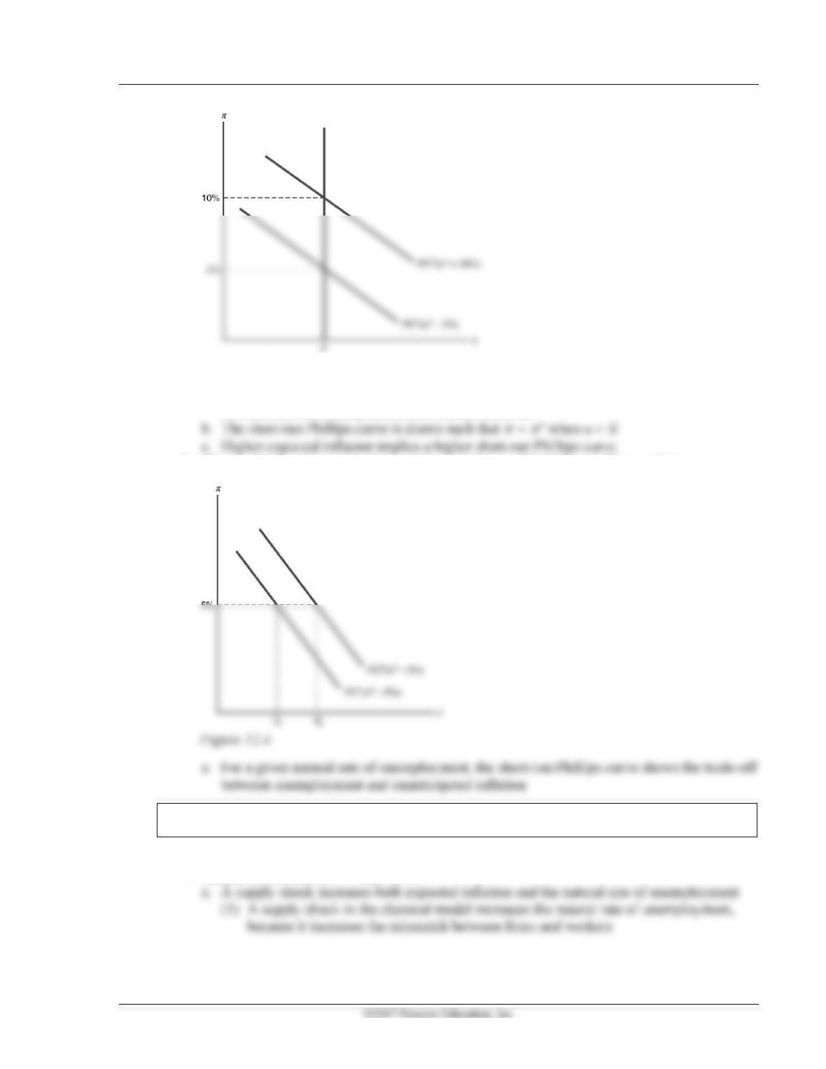
Figure 12.3

a. For a given expected rate of inflation, the short-run Phillips curve shows the trade-off

between cyclical unemployment and actual inflation

3. Changes in the natural rate of unemployment (Figure 12.4; like text Figure 12.6)

Analytical Problem 1 looks at possible ways to change the natural rate of unemployment.

b. A higher natural rate of unemployment shifts the short-run Phillips curve to the right

4. Supply shocks and the Phillips curve

(2) A supply shock in the Keynesian model reduces the marginal product of labor and

thus reduces labor demand at the fixed real wage, so the natural unemployment

5. The shifting short-run Phillips curve in practice

a. Why did the original Phillips curve relationship apply to many historical cases?

(1) The original relationship between inflation and unemployment holds up as long as

expected inflation and the natural rate of unemployment are approximately constant

II. Macroeconomic Policy and the Phillips Curve (Sec. 12.2)

A. Can the Phillips curve be exploited by policymakers? Can they choose the optimal combination

of unemployment and inflation?

1. Classical model: NO

a. The unemployment rate returns to its natural level quickly, as people’s expectations

Policy Application

The theory of rational expectations explains why the Phillips curve trade-off appeared to be stable

for some time, but failed when policymakers tried to exploit it. In the 1960s people assumed that

any rise in inflation would be temporary. But once policymakers began to exploit the trade-off,

people caught on quickly. Instead of having adaptive expectations, which were rational in the

past, people began to watch what policymakers were doing. Then expected inflation changed

quickly with changes in policy.

2. Keynesian model: YES, temporarily

a. The expected rate of inflation in the Phillips curve is the forecast of inflation at the time

Chapter 12 Unemployment and Inflation 277

Theoretical Application

The Keynesian models of the early 1970s assumed that people formed adaptive expectations, that

is, that expected inflation depended only on past inflation, so

e

t



= f (



t − 1,



t − 2, . . .). According to

B. In touch with data and research: The Lucas critique

1. When the rules of the game change, behavior changes

2. For example, if batters in baseball were called out after two strikes instead of three, they’d

swing more often when they have one strike than they do now

Theoretical Application

Robert Lucas and Tom Sargent spelled out the implications of the Lucas critique for future work

C. The long-run Phillips curve

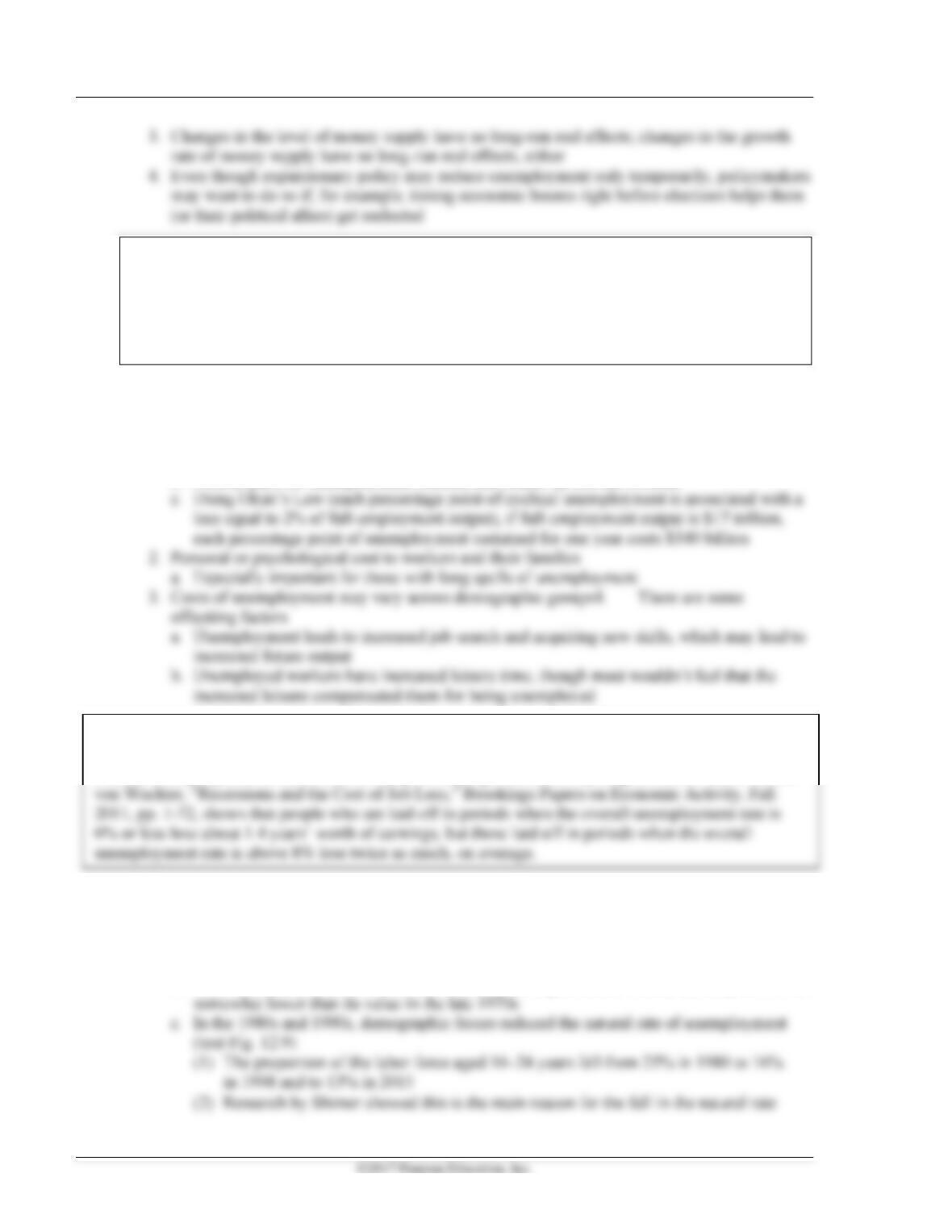
1. Long run: u =

u

for both Keynesians and classicals

u

278 Abel/Bernanke/Croushore • Macroeconomics, Ninth Edition

Theoretical Application

For a well written history of the Phillips curve and its usefulness, see the article by Robert J.

Gordon, “The Phillips Curve Now and Then,” National Bureau of Economic Research Working

Paper No. 3393, June 1990. For more recent research on the Phillips curve, see the symposium in

the Journal of Money, Credit, and Banking 39 (supplement, Feb. 2007).

III. The Problem of Unemployment (Sec. 12.3)

A. The costs of unemployment

1. Loss in output from idle resources

a. Workers lose income

b. Society pays for unemployment benefits and makes up lost tax revenue

B. The long-term behavior of the unemployment rate

1. The changing natural rate

a. How do we calculate the natural rate of unemployment?

b. CBO’s estimates: about 5.5% in 2015, somewhat higher than it was in the early 2000s but

Data Application

Recent research suggests that the costs of unemployment to individual workers may be higher if they

become unemployed at the same time as many other people. Research by Stephen J. Davis and Till M.

Chapter 12 Unemployment and Inflation 279

d. Some economists think the natural rate of unemployment was 4.5% or even lower in the

1990s and 2000s

f. Increased labor productivity may increase the natural rate of unemployment

(1) If increases in real wages lag changes in productivity, firms hire more workers and

Data Application

A very different picture of the natural rate of unemployment than that of the CBO comes from

2. Measuring the natural rate of unemployment

a. Policymakers need a measure of the natural rate of unemployment to use the

unemployment rate for setting policy

b. Economists disagree about how to measure the natural rate of unemployment and the

Analytical Problem 6 looks at events that change the natural rate of unemployment.

IV. The Problem of Inflation (Sec. 12.4)

A. The costs of inflation

1. Perfectly anticipated inflation

a. No effects if all prices and wages keep up with inflation

280 Abel/Bernanke/Croushore • Macroeconomics, Ninth Edition

Policy Application

Shoe-leather costs are generated by people’s attempt to reduce how much cash they hold.

Implicitly, inflation is like a tax on people’s cash holdings, because the government buys things

Policy Application

Two other costs of anticipated inflation are increased taxation on capital income and the

mortgage-tilt problem.

Because taxes are based on the dollar value of interest that savers receive, the higher the

inflation rate is, the larger is the government’s tax revenue as a proportion of a saver’s real

return. The increase in the government’s effective real tax rate represents a distortion to the

economy—higher anticipated inflation reduces saving and investment.

Another cost of perfectly anticipated inflation is the problem of “tilting” the real value of loan

2. Unanticipated inflation (



−



e)

a. Realized real returns differ from expected real returns

(1) Expected r = i −



e

Chapter 12 Unemployment and Inflation 281

Data Application

d. So people want to avoid risk of unanticipated inflation

(1) They spend resources to forecast inflation

Data Application

(2) In touch with data and research: Indexed contracts

(a) People could use indexed contracts to avoid the risk of transferring wealth

because of unanticipated inflation

Policy Application

It’s difficult to figure out how to index wages to inflation, or how low inflation should be, when

e. Loss of valuable signals provided by prices

(1) Confusion over changes in aggregate prices vs. changes in relative prices

(2) People expend resources to extract correct signals from prices

Data Application

For a review of the empirical evidence on the costs of inflation, see the article by John Driffill,

3. The costs of hyperinflation

a. Hyperinflation is a very high, sustained inflation (e.g., 50% or more per month)

282 Abel/Bernanke/Croushore • Macroeconomics, Ninth Edition

Data Application

There are many wonderful stories one can tell to illustrate the problems that arise in

hyperinflations. For example, there’s the story about the person who goes to the bank with a

b. There are large shoe-leather costs, as people minimize cash balances

c. People spend many resources getting rid of money as fast as possible

d. Tax collections fall, as people pay taxes with money whose value has declined sharply

e. Prices become worthless as signals, so markets become inefficient

4. Can Inflation Be Too Low?

a. Should central banks be concerned about low inflation rates or even deflation (negative

rates of inflation?)

b. Low inflation can be harmful

1. Borrowers are hurt by unexpectedly low inflation, as in the 1930s, when deflation

c. Nominal interest rates cannot generally fall below zero, so under deflation, real interest

rates cannot be very low

1. So a central bank’s ability to reduce real interest rates to combat a recession is

limited

d. What inflation rate should central banks aim for?

1. Many central banks target inflation around 2%

Chapter 12 Unemployment and Inflation 283

Policy Application

Given the costs of inflation and the vertical long-run Phillips curve, what is the optimal rate of

inflation? Some economists suggest that the optimal rate of inflation is zero or even negative

(so that the nominal rate of interest is zero). See the discussion by Michelle R. Garfinkel, “What

V. Fighting inflation: The role of inflationary expectations (Sec. 12.5)

A. If rapid money growth causes inflation, why do central banks allow the money supply to grow

rapidly?

1. Developing or war-torn countries may not be able to raise taxes or borrow, so they print

money to finance spending

Data Application

There are many problems with price indexes; they are imperfect measures of price changes. What

do the indexes do when new goods are introduced? What happens as more efficient stores replace

stores that had higher intermediate costs? How do we account for the fact that people substitute

C. The costs of disinflation could be reduced if expected inflation fell at the same time actual

inflation fell

D. Rapid versus gradual disinflation

1. The classical prescription for disinflation is cold turkey—a rapid and decisive reduction in

money growth

284 Abel/Bernanke/Croushore • Macroeconomics, Ninth Edition

(3) The strategy might fail to alter inflation expectations, because if the costs of the

policy are high (because the economy goes into recession), the government will

reverse the policy

Data Application

Tom Sargent (“The Ends of Four Big Inflations”) suggests that high rates of inflation may be

2. The Keynesian prescription for disinflation is gradualism

a. A gradual approach gives prices and wages time to adjust to the disinflation

Policy Application

In the late 1980s the Federal Reserve embarked on an attempt at gradualism, at least in their

b. Such a strategy will be politically sustainable because the costs are low

Data Application

In my article “What Are the Costs of Disinflation?” Federal Reserve Bank of Philadelphia

Business Review, May/June 1992, pp. 3–16, I examine the costs to the economy of reducing

E. In touch with data and research: The sacrifice ratio

1. When unanticipated tight monetary and fiscal policies are used to reduce inflation, they

reduce output and employment for a time, a cost that must be weighed against the benefits

of lower inflation

2. Economists use the sacrifice ratio as a measure of the costs

a. The sacrifice ratio is the number of percentage points of output lost in reducing