Economics Chapter 12 Aggregate Expenditure And Output The Short

CHAPTER 12 | Aggregate Expenditure and

Output in the Short Run

Brief Chapter Summary and Learning Objectives

The Keynesian income-expenditure approach (the “45°-line diagram” or “Keynesian cross”) is useful to

introduce students to the short-run relationship between spending and production. Many instructors,

however, prefer to omit this material. Therefore, the textbook uses the 45°-line diagram only in Chapter 12,

“Aggregate Expenditure and Output in the Short Run.” The discussion of monetary and fiscal policy in

later chapters uses only the AD-AS model, making it possible for instructors to skip Chapter 12.

12.1 The Aggregate Expenditure Model (pages 772–775)

Understand how macroeconomic equilibrium is determined in the aggregate expenditure

12.2 Determining the Level of Aggregate Expenditure in the Economy

(pages 775–789)

12.3 Graphing Macroeconomic Equilibrium (pages 789–796)

Use a 45-line diagram to illustrate macroeconomic equilibrium.

12.4 The Multiplier Effect (pages 796–803)

Describe the multiplier effect and use the multiplier formula to calculate changes in

12.5 The Aggregate Demand Curve (pages 803–805)

Understand the relationship between the aggregate demand curve and aggregate

expenditure.

▪ The aggregate demand curve shows the relationship between the price level and the level

of aggregate expenditure, holding constant all factors that affect aggregate expenditure

272 CHAPTER 12 | Aggregate Expenditure and Output in the Short Run

Appendix: The Algebra of Macroeconomic Equilibrium (pages 812–813)

Apply the algebra of macroeconomic equilibrium.

Key Terms

Aggregate demand (AD) curve, p. 804. A

curve that shows the relationship between the

price level and the level of planned aggregate

expenditure in the economy, holding constant all

other factors that affect aggregate expenditure.

Cash flow, p. 783. The difference between the

cash revenues received by a firm and the cash

spending by a firm.

Consumption function, p. 777. The relationship

between consumption spending and disposable

income.

Inventories, p. 773. Goods that have been

produced but not yet sold.

Multiplier effect, p. 797. The process by which

an increase in autonomous expenditure leads to a

larger increase in real GDP.

Chapter Outline

Fluctuating Demand Helps—and Hurts—Intel and Other Firms

Intel is the world’s largest semiconductor manufacturer and a major supplier of the microprocessors

and memory chips found in most personal computers. Because of its dependence on computer sales,

CHAPTER 12 | Aggregate Expenditure and Output in the Short Run 273

12.1

The Aggregate Expenditure Model (pages 772–775)

Learning Objective: Understand how macroeconomic equilibrium is determined in the

aggregate expenditure model.

Aggregate expenditure (AE) is total spending in the economy: the sum of consumption, planned

investment, government purchases, and net exports. The aggregate expenditure model is a

macroeconomic model that focuses on the short-run relationship between total spending and real GDP,

assuming that the price level is constant. The key idea of the model is that in any particular year, the level

of GDP is determined mainly by the level of aggregate expenditure.

A. Aggregate Expenditure

In 1936, John Maynard Keynes published The General Theory of Employment, Interest, and Money, a

We can write:

Aggregate expenditure = Consumption + Planned Investment + Government purchases + Net exports

B. The Difference between Planned Investment and Actual Investment

Inventories are goods that have been produced but not yet sold. For the economy as a whole, we can say

that actual investment spending will be greater than planned investment spending when there is an

C. Macroeconomic Equilibrium

For the economy as a whole, macroeconomic equilibrium occurs where aggregate expenditure equals total

production, or GDP:

D. Adjustments to Macroeconomic Equilibrium

When aggregate expenditure is greater than GDP, inventories will decline, and GDP and total employment

will increase. When aggregate expenditure is less than GDP, inventories will increase, and GDP and total

274 CHAPTER 12 | Aggregate Expenditure and Output in the Short Run

Teaching Tips

It will help your students understand macroeconomic equilibrium if you briefly review how equilibrium is

achieved in a market for a good or service. Remind students how price adjusts to return a market to

equilibrium if there is a shortage or surplus in a market. In contrast, in the aggregate expenditure model,

prices are constant and changes in inventories adjust to return the macroeconomy to equilibrium.

require more elaborate calculations than other problems and the use of Excel spreadsheets.

Extra Making

the

Connection

Changes in Inventory Spending Offer Preview of Future GDP

Growth

Changes in inventories are a small part of total gross domestic product. In 2014, for example, the real

value of changes in private inventories equaled $68.0 billion, less than one-half of one percent of GDP.

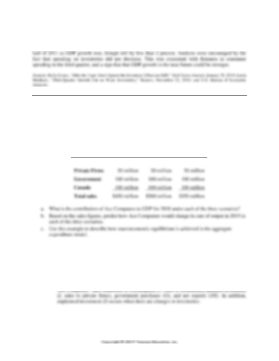
Change in Inventories

(billions of dollars, seasonally adjusted at annual rates)

2009

2010

2011

I

II

III

IV

I

II

III

IV

I

II

III

When businesses increase production to build their inventories, employment increases. As workers earn

more income, they spend more, leading to an increase in consumption, which is the largest component of

GDP. “That’s how recoveries become self-sustaining,” says Dean Maki, chief U.S. economist at Barclays

CHAPTER 12 | Aggregate Expenditure and Output in the Short Run 275

The increase in inventories that continued through the third quarter of 2011 coincided with increases in

the growth rate of real GDP. But GDP growth stalled in 2011, rising only 0.4 percent in the first quarter,

leading some to wonder if the economy was heading to another recession. These fears faded in the second

Extra Solved Problem 12.1

Ace Computers and Aggregate Expenditure

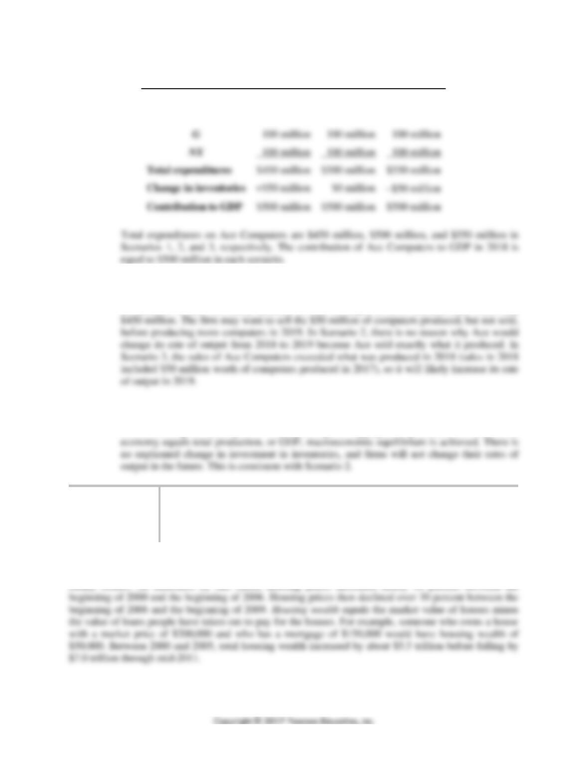
Suppose that Ace Computers, Inc., produces $500 million of new computers in 2018. Ace sells computers

to households, private firms, and local and state government agencies. Some of Ace’s sales are to

households, firms, and government agencies in Canada. The following table represents three different

scenarios for Ace Computers’ sales.

Sales to:

Scenario 1

Scenario 2

Scenario 3

Households

$200 million

$250 million

$300 million

Canada

100 million

Solving the Problem

Step 1: Review the chapter material.

This problem is about aggregate expenditure, so you may want to review the section “The

Aggregate Expenditure Model,” which begins on page 772 in the textbook.

Step 2: Explain Ace Computer’s contribution to GDP for 2018 under each of the scenarios.

276 CHAPTER 12 | Aggregate Expenditure and Output in the Short Run

Scenario 1

Scenario 2

Scenario 3

C

$200 million

$250 million

$300 million

I

50 million

G

100 million

$500 million

Step 3: Use the sales figures to predict how Ace Computers would change its rate of

output in 2019 in each of the three scenarios.

In Scenario 1, Ace will likely decrease its rate of output in 2019 because sales were only

Step 4: Use the Ace Computers example to describe how macroeconomic equilibrium is

achieved in the aggregate expenditure model.

When for a given time period total spending, or aggregate expenditure, for the entire

Extra Making

the

Connection

Do Changes in Housing Wealth Affect Consumption Spending?

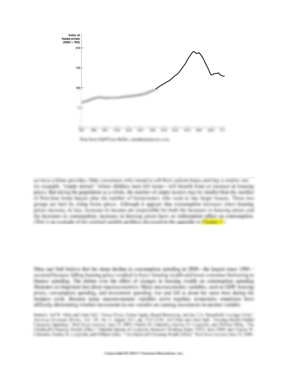
From 2000 to 2006, housing prices increased sharply in many parts of the United States. The figure below

shows the S&P/Case-Shiller index of housing prices, which represents changes in the prices of single–

family homes. As measured by this index, housing prices increased nearly 90 percent between the

CHAPTER 12 | Aggregate Expenditure and Output in the Short Run 277

Did these big swings in housing wealth affect consumption spending? Economists are divided in their

opinions. Charles Calomiris of Columbia University, Stanley Longhofer of the Barton School of

Business, and William Miles of Wichita State University argue that changes in housing wealth have little

or no effect on consumption. They argue that consumers do not consider houses to be assets similar to

their holdings of stocks and bonds because they own houses primarily so they can consume the housing

Atif Mian and Amir Sufi, both of the University of Chicago, strongly disagree with Calomiris, Longhofer,

and Miles. Mian and Sufi tracked a sample of 70,000 consumers from 1998 to 2008 and found that

consumers living in cities that experienced dramatic increases in housing prices borrowed heavily as their

housing wealth increased. Consumers used these borrowed funds to increase their spending on goods and

services.

278 CHAPTER 12 | Aggregate Expenditure and Output in the Short Run

Question

Writing about the state of the British economy, an article in the Economist argued: “Spending will be

hit…by weak stock–markets and shrinking housing wealth.” Would Calomiris, Longhofer, and Miles

agree with this argument? Would Mian and Sufi? Briefly explain.

Source: “Combating the Recession,” Economist, January 8, 2009.

Answer

Calomiris, Longhofer, and Miles would disagree with this argument because they believe that changes in

12.2

Determining the Level of Aggregate Expenditure in the Economy

(pages 775–789)

Learning Objective: Discuss the determinants of the four components of aggregate

expenditure and define marginal propensity to consume and marginal propensity to save.

There are four components of aggregate expenditure. Each component is measured in real terms.

Consumption is the largest component of aggregate expenditure.

A. Consumption

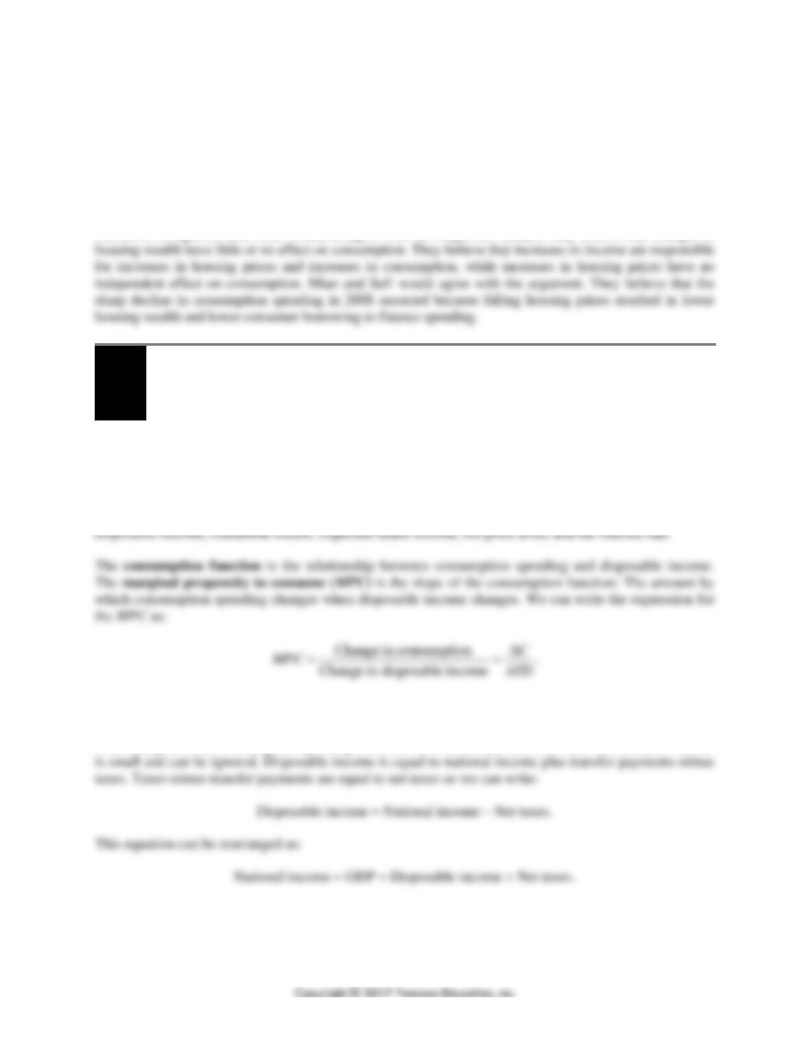
The following are the five most important variables that determine the level of consumption: current

B. The Relationship between Consumption and National Income

Consumption spending by households depends on disposable income, but we want to focus on the

relationship between consumption spending and GDP. The difference between GDP and national income

CHAPTER 12 | Aggregate Expenditure and Output in the Short Run 279

C. Income, Consumption, and Saving

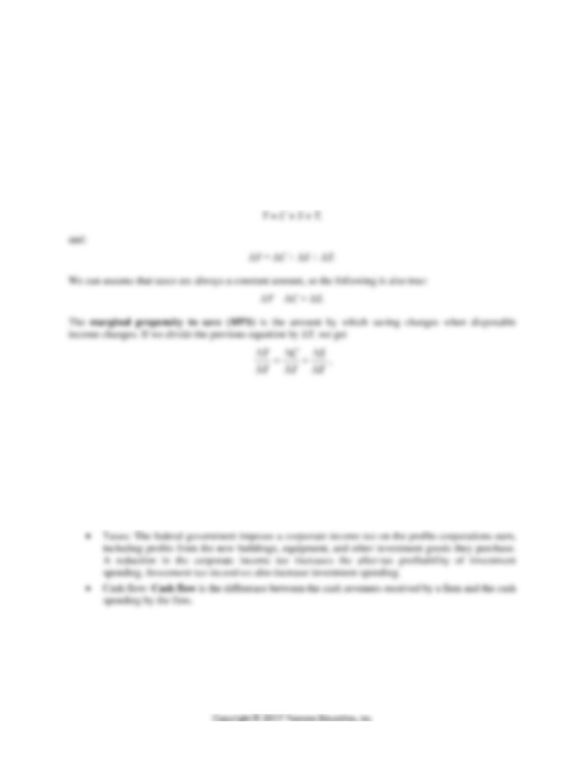
For the economy as a whole:

National income = Consumption + Saving + Taxes.

When national income increases, there must be a combination of increases in consumption, saving, and

taxes:

Change in national income = Change in consumption + Change in saving + Change in taxes.

Using symbols, where Y represents national income (and GDP), C represents consumption, S represents

saving and T represents taxes, we can write:

or

1 = MPC + MPS.

This equation tells us that when taxes are constant, the marginal propensity to consume plus the marginal

propensity to save must always equal 1.

D. Planned Investment

The four most important variables that determine the level of investment are:

• Expectations of future profitability

• The interest rate

E. Government Purchases

Total government purchases include all spending by federal, state and local governments for goods and

services.

280 CHAPTER 12 | Aggregate Expenditure and Output in the Short Run

F. Net Exports

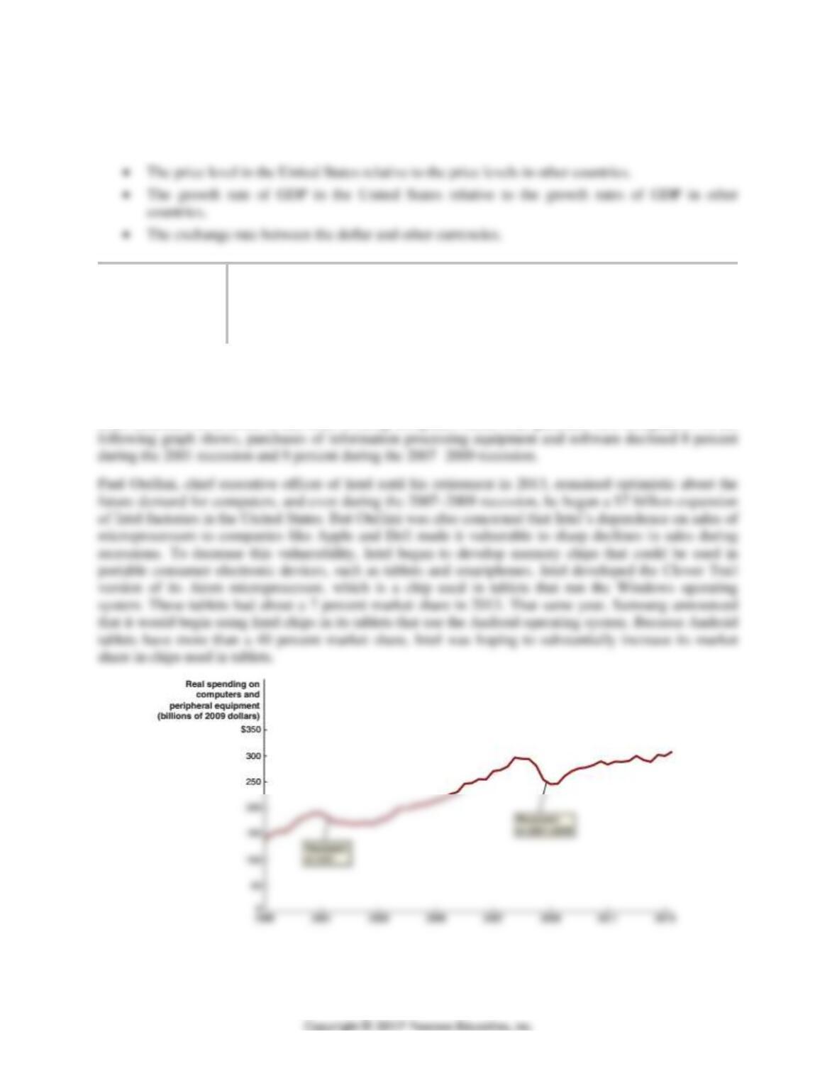
Net exports equal exports minus imports. The three most important variables that determine the level of

net exports are:

Extra Making

the

Connection

Intel Moves into Tablets and Perceptual Computing

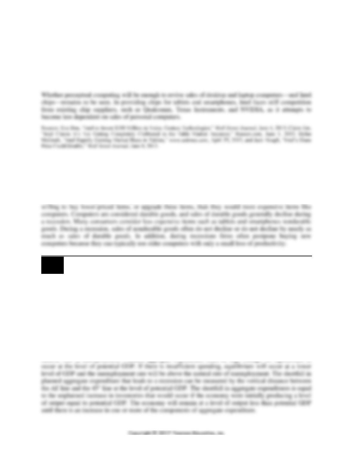
We saw in the chapter opener that Intel has a large market share in microprocessors that companies such

as Apple and Dell use in their computers. Spending on durable goods, like computers, follows the

business cycle. During recessions, firms and households reduce spending on computers because they can

often continue for a while to use their existing computers rather than purchase new computers. As the

CHAPTER 12 | Aggregate Expenditure and Output in the Short Run 281

Intel also encouraged hardware and software developers with innovations in perceptual computing, which

allows users to interact with computers through speaking, gesturing with hands and fingers, or changing

facial expressions. Intel entered a partnership with Creative Technologies to develop a 3-D camera that

was available in late 2013 and helped support perceptual computing. It also started a $100 million fund,

which one Intel executive described as an attempt to “find companies that have those kinds of innovative

breakthroughs and help get them to work.”

Question

We saw that Intel hopes to increase sales of microprocessors used in tablets and smartphones. During a

recession, why would spending on these products be more stable than spending on computers?

Answer

Tablets and smartphones sell at lower prices than do computers, and the quantity of these items produced

and sold is much larger than the quantity of computers. During a recession, consumers would be more

12.3

Graphing Macroeconomic Equilibrium (pages 789–796)

Learning Objective: Use a 45-line diagram to illustrate macroeconomic equilibrium.

We can use a 45°-line diagram to illustrate macroeconomic equilibrium. In a graph, the line represents all

the points that are equal distances from both axes. Since macroeconomic equilibrium occurs where

planned aggregate expenditure equals GDP, we know that all points of macroeconomic equilibrium must

lie along the 45° line. We assume that the variables that determine planned investment, government

purchases, and net exports all remain constant, as well as the variables other than GDP that affect

consumption. Where the aggregate expenditure (AE) line crosses the 45° line, planned aggregate

expenditure is equal to GDP, and the economy is in macroeconomic equilibrium.

A. Showing a Recession on the 45-Line Diagram

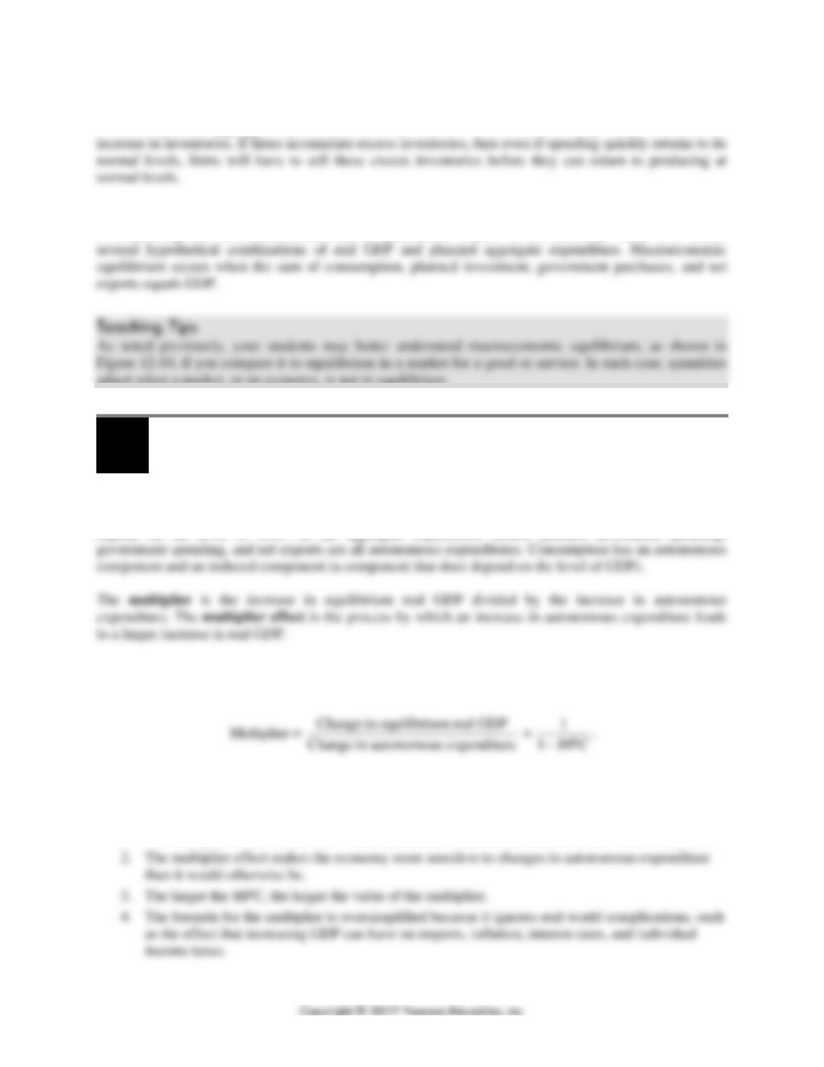
At potential GDP, firms will be operating at their normal level of capacity, and the economy will be at the

natural rate of unemployment. Planned aggregate expenditure must be high enough for equilibrium to

282 CHAPTER 12 | Aggregate Expenditure and Output in the Short Run

B. The Important Role of Inventories

Whenever planned aggregate expenditure is less than real GDP, some firms will experience an unplanned

C. A Numerical Example of Macroeconomic Equilibrium

In forecasting real GDP, economists rely on quantitative models of the economy. Table 12.3 shows

adjust when a market, or an economy, is not in equilibrium.

12.4

The Multiplier Effect (pages 796–803)

Learning Objective: Describe the multiplier effect and use the multiplier formula to

calculate changes in equilibrium GDP.

Any increase in autonomous expenditure will shift up the aggregate expenditure function and lead to a

multiplied increase in equilibrium real GDP. Autonomous expenditure is an expenditure that does not

depend on the level of GDP. In the aggregate expenditure model, planned investment spending,

A. A Formula for the Multiplier

The general formula for the multiplier is:

B. Summarizing the Multiplier Effect

There are four key points about the multiplier effect:

1. The multiplier effect occurs both when autonomous expenditure increases and when it decreases.

CHAPTER 12 | Aggregate Expenditure and Output in the Short Run 283

C. The Paradox of Thrift

In the short run, if households save more of their income and spend less of it, aggregate expenditure and

real GDP will decline. John Maynard Keynes argued that if many households decide at the same time to

12.5

The Aggregate Demand Curve (pages 803–805)

Learning Objective: Understand the relationship between the aggregate demand curve

and aggregate expenditure.

We expect that an increase or decrease in aggregate expenditure will affect both real GDP and the price

level. There are three reasons why there is an inverse relationship between changes in the price level and

changes in aggregate expenditure.

• A rising price level decreases consumption by decreasing the real value of household wealth; a

falling price level has the reverse effect.

Extra Solved Problem 12.5

Do Price Changes Affect Aggregate Expenditure?

When studying demand and supply, you learn that a price change is considered the most important

determinant of the quantity demanded for a good or service. It may seem odd that in discussing

the determinants of total spending or aggregate expenditure, the textbook states that the most important

determinant of consumption is the current disposable income of households. If changes in price are

important determinants of consumption in individual markets, why aren’t they important in determining

284 CHAPTER 12 | Aggregate Expenditure and Output in the Short Run

Changes in aggregate expenditure are related to changes in the price level. Economists use an aggregate

demand (AD) curve to analyze this relationship. This curve shows the relationship between the level of

planned expenditure and the price level, holding constant other factors such as interest rates and wealth

Solving the Problem

Step 1: Review the chapter material.

This problem is about the relationship between the aggregate demand curve and aggregate

expenditure, so you may want to review the section “The Aggregate Demand Curve,” which

begins on page 803 in the textbook.

Step 2: Explain why if relative prices do not fall as the price level falls, there is an

increase in consumption.

The increase in consumption can be explained by the increase in purchasing power

Extra Making

the

Connection

“Made in China” (and the United States)

In recent years many politicians, business managers, and ordinary citizens have expressed concern about

the increasing amounts of goods sold in the United States with a “Made in China” label. This concern has

Fact # 1: Many U.S. Firms Export to China

From 1990 to 2012, China rose from the eighteenth to the third largest market for U.S. exports, including

goods such as semiconductors, aircraft, industrial machinery, copper, and chemicals. Exports from the

U.S. to China grew 294 percent from 2003 to 2012. The Paulson Manufacturing Corp., a maker of facial

CHAPTER 12 | Aggregate Expenditure and Output in the Short Run 285

Fact # 2: Chinese Imports Are a Small Percentage of U.S. GDP

Galina Hale and Bart Hobijn, economists at the Federal Reserve Bank of San Francisco, found that

Fact # 3: A Significant Fraction of Spending for Chinese Imports Benefits U.S. Companies

Hale and Hobijn estimate that 55 cents of every dollar spent on an item with a “Made in China” label is

spent on services—transportation, wholesale and retail activities—produced in the United States. This is

Extra Economics in Your Life:

Will Lower Net Exports Jeopardize Your Job?

Question: Suppose you are a customer service representative of a large computer company and you

read the following headline in your newspaper: “U.S. exports in July increased less than U.S. imports.”

Should you be concerned about losing your job?

Extra AN INSIDE LOOK News Article to Use in Class