Chapter 12 Unemployment and Inflation 285
4. Ball’s results should be interpreted with caution, since it isn’t easy to calculate the loss
of output and because supply shocks can distort the calculation of the sacrifice ratio
Data Application
A version of Ball’s article that is accessible to students is “How Costly Is Disinflation? The
F. Wage and price controls
1. Pro: Controls would hold down inflation, thus lowering expected inflation and reducing the
costs of disinflation
b. If tight policies are pursued, expected inflation may decline
Analytical Problem 5 looks at what happens if the government uses wage and price controls, but
continues to use expansionary policies.
4. The Nixon wage-price controls from August 1971 to April 1974 led to shortages in many
products; the controls reduced inflation when they were in effect, but prices returned to
where they would have been soon after the controls were lifted
G. Credibility and reputation
1. Key determinant of the costs of disinflation: how quickly expected inflation adjusts
H. The U.S. disinflation of the 1980s and 1990s
1. Fed chairmen Volcker and Greenspan gradually reduced the inflation rate in the 1980s and
1990s
5. To solidify those expectations, the Fed declared a 2% long-run inflation target in 2012

286 Abel/Bernanke/Croushore • Macroeconomics, Ninth Edition
Data Application
In the severe recession that began in December 2007 and was precipitated by the housing crisis,
inflation declined substantially. Some analysts thought that inflation fell mainly because of the
Chapter 12 Unemployment and Inflation 287
◼ Additional Issues for Classroom Discussion
1. Additional Costs of Anticipated Inflation
The interaction of the tax system with inflation. Most countries’ tax systems are not perfectly
indexed for inflation. They impose taxes on nominal, not real, returns on investments (bonds and stocks),
which distort the prices on those assets. Also, capital gains are taxed in nominal terms, so investors may
pay a big tax on assets whose value hasn’t even increased in real terms. Eytan Sheshinski, in “Treatment
The mortgage tilt problem. Mortgage loans are most often made at fixed rates for long terms. When
inflation is positive, the constant nominal payment over time is much higher in real terms early in the life of
the loan, and lower in real terms later in the life of the loan, because of a higher price level. This means that
the burden of paying the loan is higher when households are younger. So if the households are liquidity
2. Can Unemployment Help Workers and the Economy?
If an unemployed worker always accepted the first job offered, unemployment would decrease in the short
run. However, such a practice is likely to reduce output and to lead to more frequent periods of
288 Abel/Bernanke/Croushore • Macroeconomics, Ninth Edition
3. Should the Fed Aim for Zero Inflation?
Discuss with your students the ultimate goal of the Federal Reserve (or any other country’s central bank).
Should the goal be to drive inflation to zero? Why is zero the best point to be? Is it good enough for
inflation to be close to zero, but positive, if it’s low and steady?
Here are some things to consider.
Second, if the inflation rate is mismeasured (see the discussion of the bias in the CPI in Chapter 2), that
should affect the Fed’s target. If the CPI inflation rate is overstated by 1 to 2 percentage points per year,
then a true target of zero inflation corresponds to measured inflation of 1 to 2 percent.
Third, what are the costs and benefits of reducing inflation? Is achieving lower inflation worth the costs?
Calculations of the sacrifice ratio suggest that to permanently reduce inflation by one percentage point
costs the economy 2 to 3 percentage points of lost output. That’s the cost of the transition to lower inflation.
Chapter 12 Unemployment and Inflation 289
◼ Answers to Textbook Problems
Review Questions
1. The Phillips curve is an empirical negative relationship between inflation and unemployment. The
Phillips curve relationship held for U.S. data in the 1960s, but broke down in the 1970s and 1980s.
2. In the original Phillips curve, inflation itself is related to the unemployment rate. In the expectations-
augmented Phillips curve, it is unanticipated inflation (the difference between actual
3. In the early 1960s the rate of inflation was fairly low (about 1% to 2%), and it didn’t vary much from
year to year. But supply shocks hit the economy in both the mid- and the late-1970s, causing a rise in
4. According to the classical point of view, the economy adjusts quickly to changes in inflation, so there
is only a very short period in which unemployment changes because of a change in inflation. Further,
5. Policymakers want to keep inflation low because inflation imposes costs on the economy. Costs of
anticipated inflation include shoe leather costs and menu costs. Costs of unanticipated inflation
6. The natural rate of unemployment is the rate of unemployment that exists when output is at its full–
employment level. This occurs when the only unemployment is frictional and structural, not cyclical.
The natural rate is crucial in understanding the Phillips curve.
The natural rate of unemployment has moved higher over time in the United States and Europe due to
290 Abel/Bernanke/Croushore • Macroeconomics, Ninth Edition
7. Two costs of anticipated inflation are shoe-leather costs and menu costs. Two costs of unanticipated
inflation are transfers of wealth and confusion of price signals.
8. The greatest potential cost of disinflation is that it may cause a recession. This occurs because
inflation may fall below expected inflation, causing the unemployment rate to rise along
9. One approach to disinflation is a cold turkey strategy. It has the advantage of reducing inflation
quickly, but it may have high costs from increasing unemployment, according to Keynesians.
10. The Federal Reserve works hard to establish its credibility so that the costs of reducing inflation
Chapter 12 Unemployment and Inflation 291
Numerical Problems
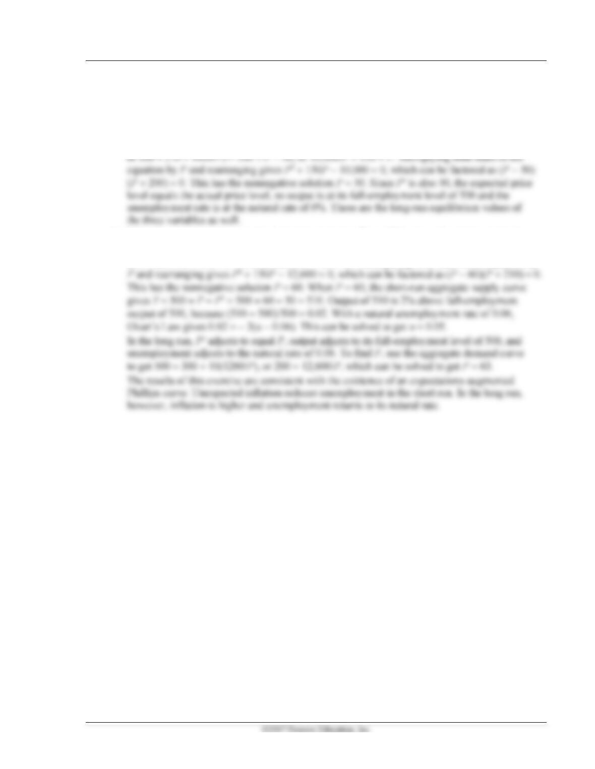
1. (a) Equating aggregate demand to short-run aggregate supply gives: 300 + 10(M/P) = 500 + P − Pe,
(b) When the nominal money supply increases unexpectedly to 1260, we again equate aggregate
demand to short-run aggregate supply, which gives: 300 + 10(M/P) = 500 + P − Pe, or 300 +
(10 1260/P) = 500 + P − 50, or 12,600/P = 150 + P. Multiplying both sides of the equation by
292 Abel/Bernanke/Croushore • Macroeconomics, Ninth Edition
2. (a)
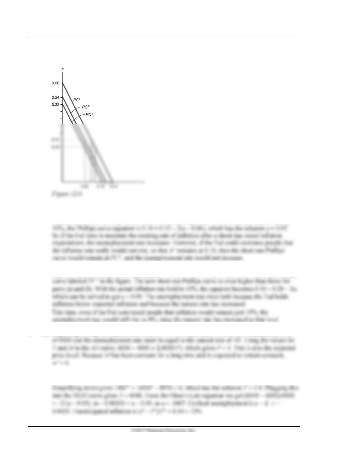
= 0.10 − 2(u − 0.06) = 0.22 − 2u. This is shown as the Phillips curve labeled PCa in Figure 12.6.
If the Fed keeps inflation at 0.10, then u = 0.06, the natural rate of unemployment.
(b) With expected inflation rising to 12%, the Phillips curve is
= 0.12 – 2(u – 0.06) = 0.24 – 2u.
This is the Phillips curve labeled PCb in the figure. The higher rate of expected inflation has
caused the curve to shift up relative to where it was in part (a). With the actual inflation rate at
(c) With the natural rate of unemployment rising to 0.08 at the same time that expected inflation
rises to 0.12, the Phillips curve equation is
= 0.12 − 2(u − 0.08) = 0.28 − 2u. This is the Phillips
3. (a) Beginning in long-run equilibrium, with M = 4000, output must be at its full-employment level
(b) With Pe = 4, the SRAS curve is Y = 6000 + 100(P − 4). The AD curve is Y = 4000 + 2(4488/P).
The intersection of the two curves occurs when 6000 + 100(P − 4) = 4000 + 2(4488/P).
Chapter 12 Unemployment and Inflation 293
4. Since the natural rate of unemployment is 0.06,
=
e − 2(u − 0.06), so u − 0.06 = 0.5(
e −
),
or u = 0.06 + 0.5(
e −
).
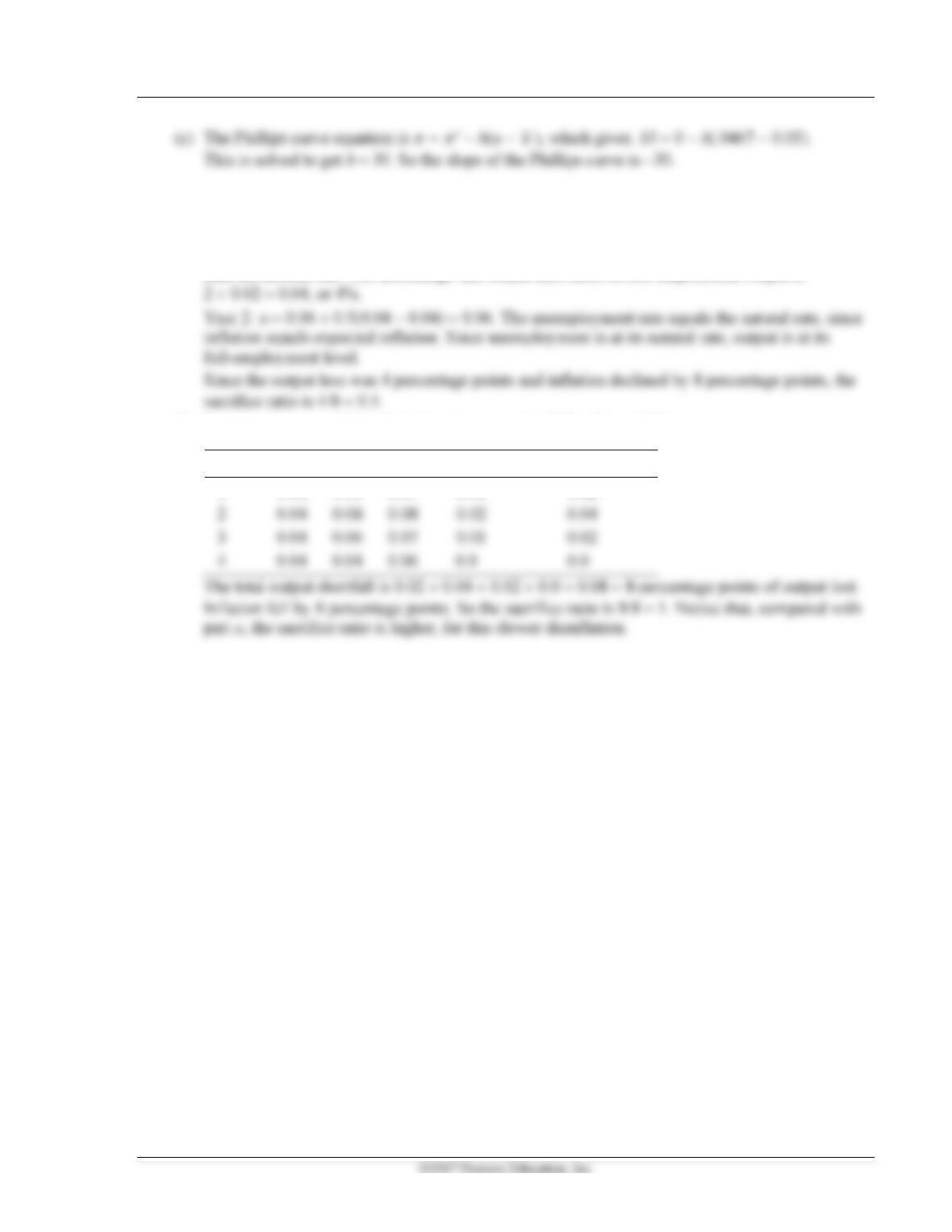
(a) Year 1: u = 0.06 + 0.5(0.08 − 0.04) = 0.06 + 0.02 = 0.08. The unemployment rate is 0.02 higher
than the natural rate. The percentage that output falls short of full-employment output is
(b) Use equations: u = 0.06 + 0.5(
e –
), output shortfall = 2 (u – 0.06).
Year
e
u
u − 0.06
Output Shortfall
1
0.08
0.10
0.07
0.01
0.02
294 Abel/Bernanke/Croushore • Macroeconomics, Ninth Edition
Analytical Problems
1. (a) The reduction in structural unemployment would reduce the natural rate of unemployment and
thus would shift both the expectations-augmented Phillips curve and the long-run Phillips curve
2. The slope of the short-run aggregate supply curve will be much steeper in economy B, because
producers increase their output only a small amount in response to an increase in price. But economy
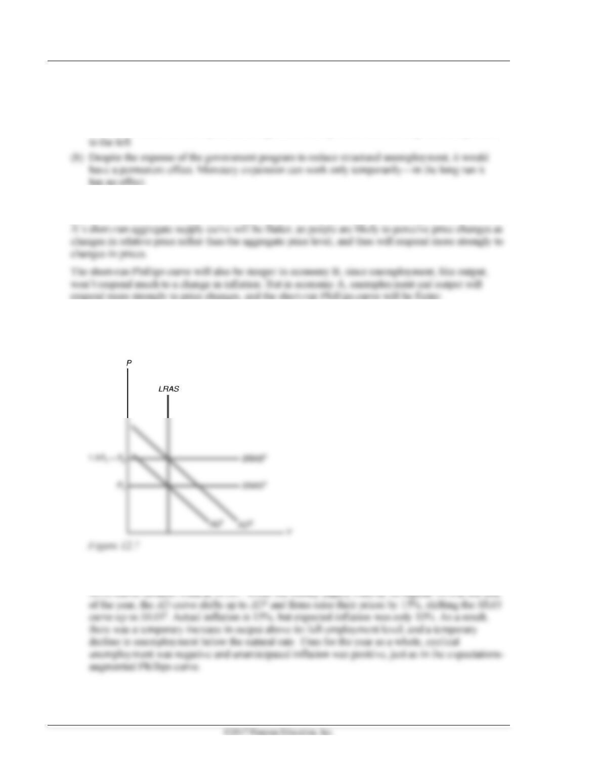
3. (a) In Figure 12.7, the SRAS curve shifts up 10% each year, as does the AD curve. Unanticipated
inflation is zero, as both actual and expected inflation are 10%. The economy is at full employment,
since firms set their prices to exactly match the increase in the general price level.
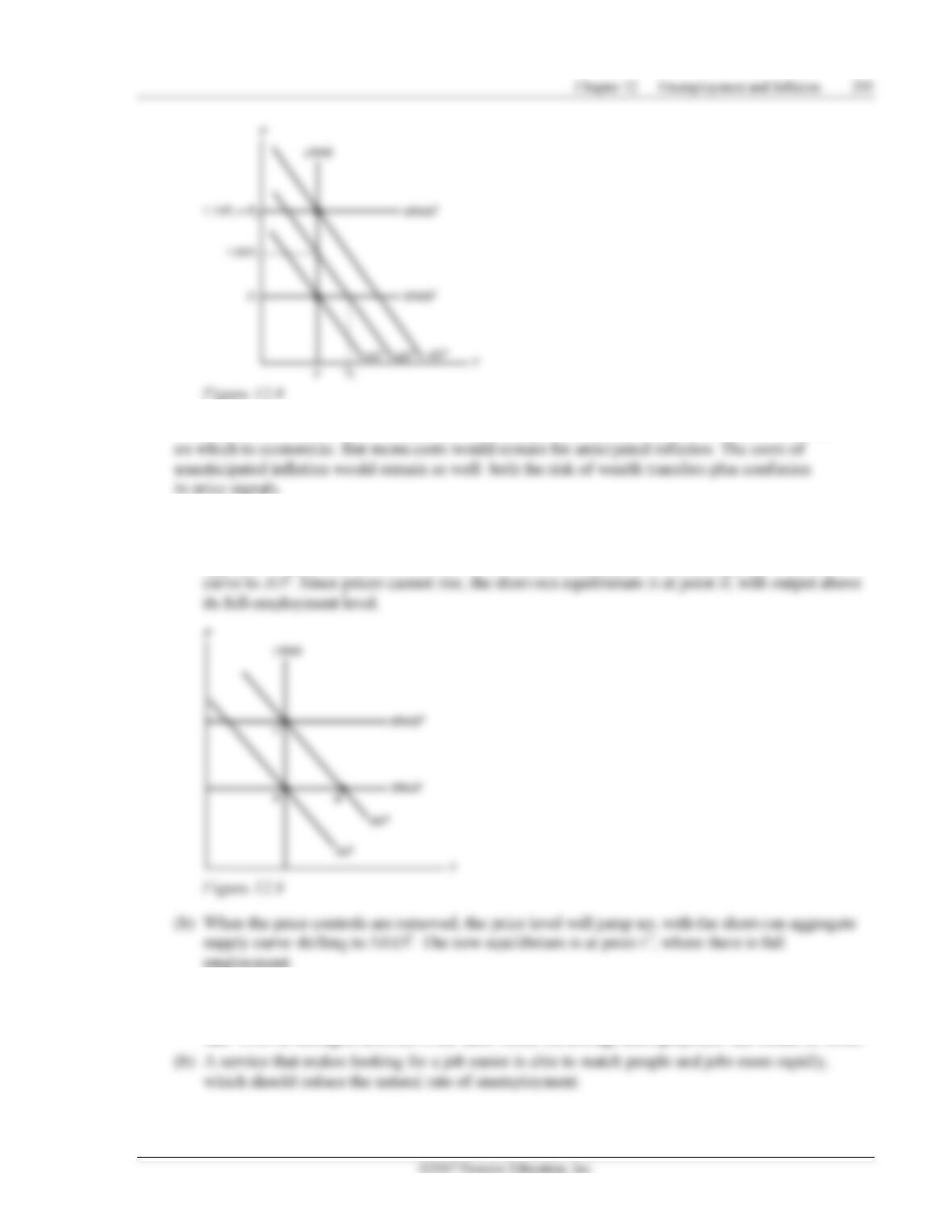
(b) The surprise increase in the money supply at mid-year leads to a rise in output, as shown in
Figure 12.8 by the shift of the AD curve from AD1 to AD2. Firms don’t adjust their prices, so the
4. In the cashless society, there would be no shoe-leather costs, as there would be no cash balances
5. (a) Figure 12.9 shows the effects of increasing the money supply while holding the price level
constant. Beginning at point A, the intersection of aggregate demand curve AD1 and short-run
aggregate supply curve SRAS1, the increase in the money supply shifts the aggregate demand
6. (a) A new law that prohibits people from seeking employment before age eighteen is likely to reduce
the natural rate of unemployment because teenagers have a higher-than-average unemployment
rate. With no teenagers allowed in the labor force, the average unemployment rate would be lower.
296 Abel/Bernanke/Croushore • Macroeconomics, Ninth Edition
(c) If unemployed workers can receive benefits longer, they’ll be in less of a rush to take a job, so
the job-matching process will take longer. As a result, the natural rate of unemployment will rise.
Working with Macroeconomic Data
1. a. Inflation and unemployment are positively related.
b. Inflation and cyclical unemployment show no apparent relationship.
2. A line through the origin with a slope of 2 is very close to the points on the line, confirming
Okun’s law.
3. The fraction of unemployed workers who have been unemployed 15 weeks or more usually
rises in recessions and continues rising for a time after recessions end. The fraction of