
CHAPTER 11
TEACHING NOTES
Much of the material in this chapter is usually postponed, or not covered at all, in an introductory
course. However, as Chapter 10 indicates, the set of time series applications that satisfy all of
the classical linear model assumptions might be very small. In my experience, spurious time
When the data are weakly dependent and the explanatory variables are contemporaneously
exogenous, OLS is consistent. This result has many applications, including the stable AR(1)
regression model. When we add the appropriate homoskedasticity and no serial correlation
assumptions, the usual test statistics are asymptotically valid.
Section 11.4 is novel in an introductory text, and simply points out that, if a model is
dynamically complete in a well-defined sense, it should not have serial correlation. Therefore,
we need not worry about serial correlation when, say, we test the efficient market hypothesis.
Section 11.5 further investigates the homoskedasticity assumption, and, in a time series context,
130
SOLUTIONS TO PROBLEMS
11.1 Because of covariance stationarity,
0
= Var(xt) does not depend on t, so sd(xt+h) =
0
for
11.2 (i) E(xt) = E(et) – (1/2)E(et–1) + (1/2)E(et-2) = 0 for t = 1,2, Also, because the et are
(ii) Because xt has zero mean, Cov(xt,xt+1) = E(xtxt+1) = E[(et – (1/2)et-1 + (1/2)et-2)(et+1 –
(iii) Corr(xt,xt+h) = 0 for h >2 because, for h > 2, xt+h depends at most on et+j for j > 0, while
11.3 (i) E(yt) = E(z + et) = E(z) + E(et) = 0. Var(yt) = Var(z + et) = Var(z) + Var(et) +
(ii) We assume h > 0; when h = 0 we obtain Var(yt). Then Cov(yt,yt+h) = E(ytyt+h) = E[(z +
(iii) From Problem 11.1 and parts (i) and (ii), Corr(yt,yt+h) = Cov(yt,yt+h)/Var(yt) =
2
z
/(
2
z
+
2
e
) > 0.
131
11.4 Assuming y0 = 0 is a special case of assuming y0 nonrandom, and so we can obtain the
variances from (11.21): Var(yt) =
2
e
t and Var(yt+h) =
2
e
(t + h), h > 0. Because E(yt) = 0 for all
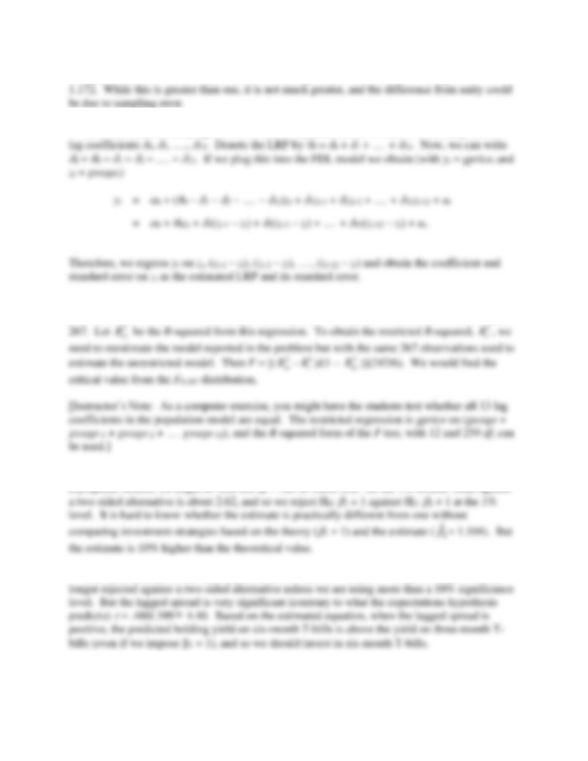
11.5 (i) The following graph gives the estimated lag distribution:
(ii) Lags two, three, and twelve have t statistics less than two. The other lags are statistically
coefficient
.12
.16
132
(iii) The estimated LRP is just the sum of the lag coefficients from zero through twelve:
(iv) The model underlying and the estimated equation can be written with intercept 0 and
(v) We would add lags 13 through 18 of gwaget to the equation, which leaves 273 – 6 = 267
observations. Now, we are estimating 20 parameters, so the df in the unrestricted model is dfur =
11.6 (i) The t statistic for H0:
1 = 1 is t = (1.104 – 1)/.039
2.67. Although we must rely on
asymptotic results, we might as well use df = 120 in Table G.2. So the 1% critical value against
(ii) The t statistic for the null in part (i) is now (1.053 – 1)/.039
1.36, so H0:
1 = 1 is no
(iii) This suggests unit root behavior for {hy3t}, which generally invalidates the usual t–
testing procedure.
133
11.7 (i) We plug the first equation into the second to get
(ii) An OLS regression of yt on yt-1 and xt produces consistent, asymptotically normal
estimators of the j. Under E(et|xt,yt-1,xt-1, ) = E(at|xt,yt-1,xt-1, ) = 0 it follows that
11.8 (i) Sequential exogeneity does not rule out correlation between, say,
1t
u−
and
tj
x
1t
u−
for any
regressors j = 1, 2, …, k. The differencing generally induces correlation between the differenced
(ii) Strict exogeneity of the regressors in the original equation is sufficient for OLS on the
(iii) If we assume sequential exogeneity in a static model, the condition can be written as
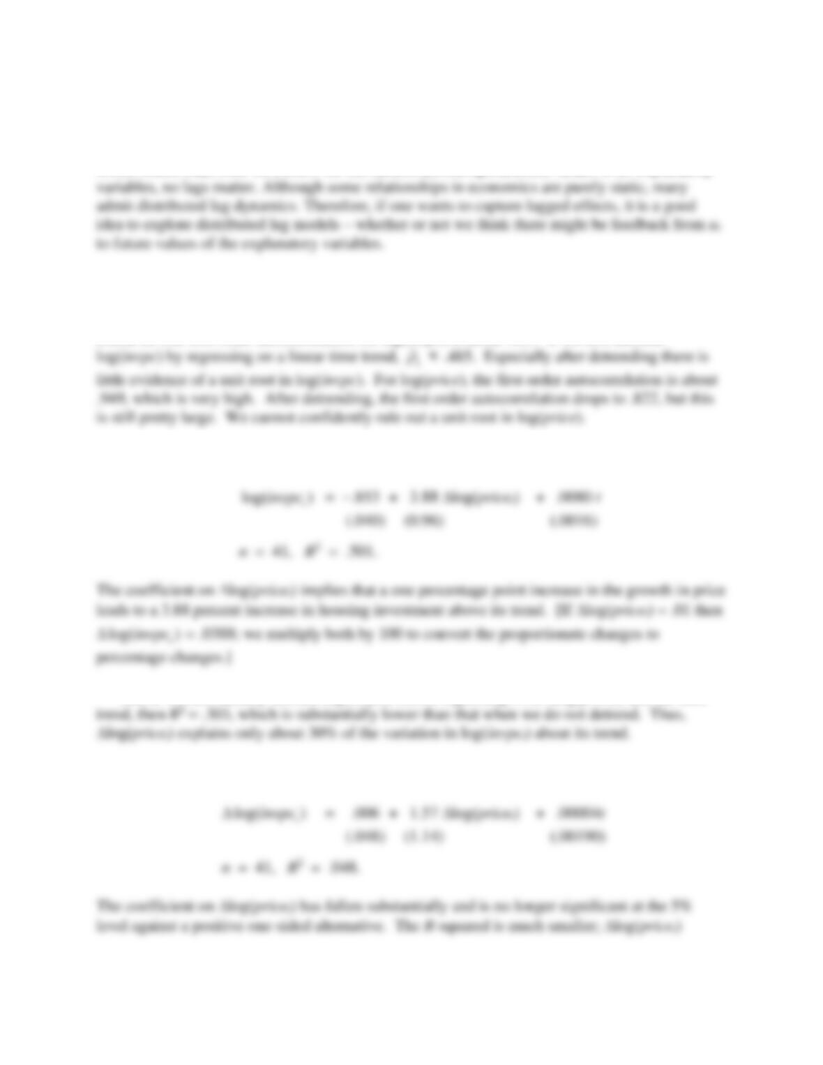
134
12
E( | , , ,…) E( | )
t t t t t t
yy
−− =z z z z
which means that, once we control for the current (comtemporaneous) values of all explanatory
SOLUTIONS TO COMPUTER EXERCISES
C11.1 (i) The first order autocorrelation for log(invpc) is about .639. If we first detrend
(ii) The estimated equation is
(iii) If we first linearly detrend log(invpct) before regressing it on log(pricet) and the time
(iv) The estimated equation is
135
C11.2 (i) The estimated equation is
The t statistic on the lag is about 2.76, so the lag is very significant.
(ii) We follow the hint and write the LRP as
=
1 +
2, and then plug
1 =
–
2 into the
original model:
C11.3 (i) The estimated equation is
(iii) When we put returnt-1
returnt-2 in place of
21t
return −
the null can still be stated as in part
136
(iv) Predicting returnt based on past returns does not appear promising. Even though the F
statistic from part (ii) is almost significant at the 10% level, we have many observations. We
cannot even explain 1% of the variation in returnt.
C11.4 (i) The estimated equation in first differences is
(ii) Based on the R-squareds (or adjusted R-squareds), the model from part (i) explains inf
C11.5 (i) The estimated equation is
The time trend coefficient is very insignificant, so it is not needed in the equation.
(ii) The estimated equation is
(iii) Including the time trend and the two dummy variables gives
137
The time trend coefficient is more than 10 times as large as when it appears by itself in part (i),
and it is now statistically significant. The magnitude on the pill coefficient has also gone way up,
and its t statistic is greater than three in absolute value.
(iv) From the equation in part (iii), with the distributed lag coefficients rounded to three
C11.6 (i) The estimated accelerator model is
(ii) When we add r3t, we obtain
138
If r3t is used instead, the coefficient becomes about −.470, se = 1.540. So this is even less
significant than when r3t is in the equation. But, without more data, we cannot conclude that
interest rates have a ceteris paribus effect on inventory investment.
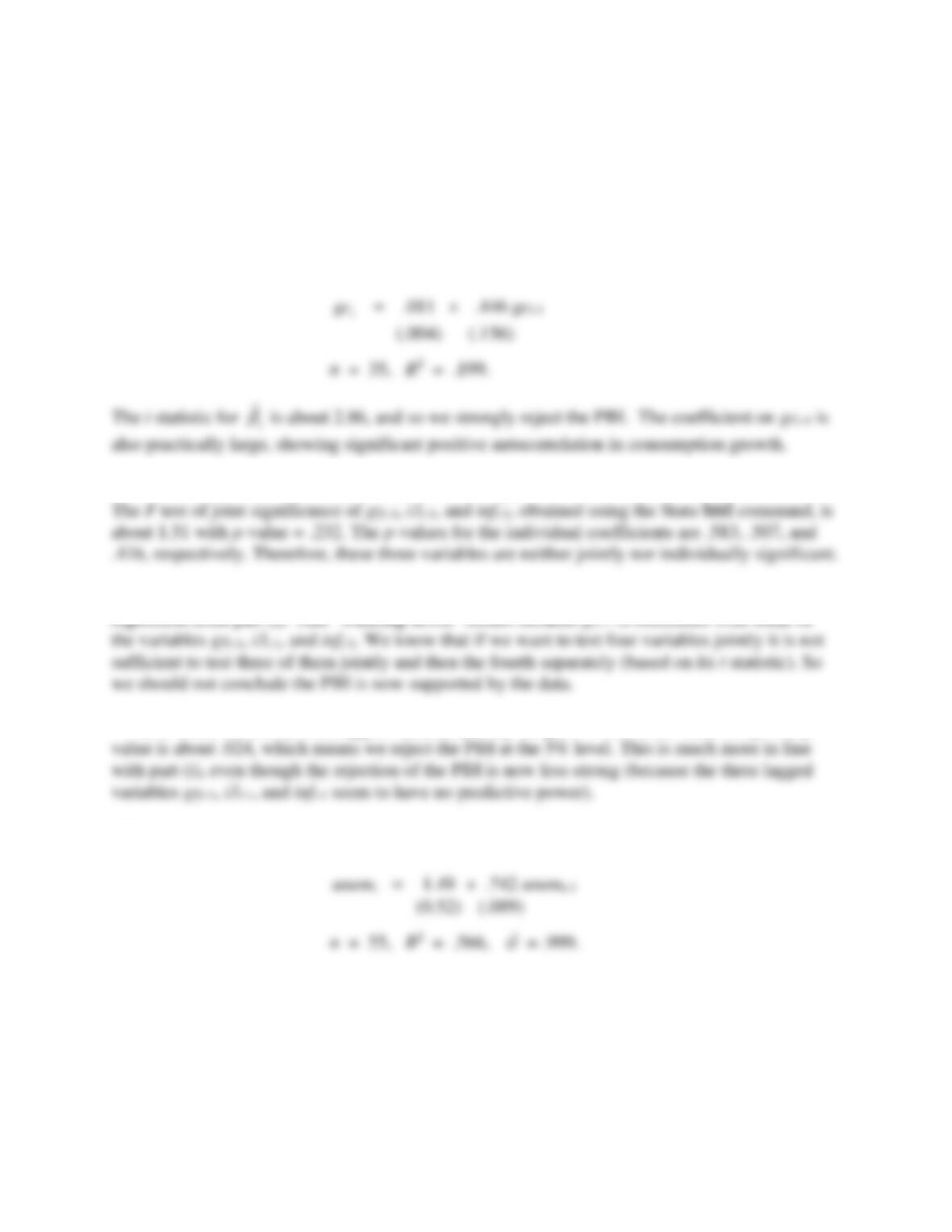
C11.7 (i) If E(gct|It-1) = E(gct) – that is, E(gct|It-1) = does not depend on gct-1, then
1 = 0 in gct =
0 +
1gct-1 + ut. So the null hypothesis is H0:
1 = 0 and the alternative is H1:
1 0. Estimating
the simple regression using the data in CONSUMP.RAW gives
(ii) When gyt-1, i3t-1, and inft-1 are added to the regression, the R-squared becomes about .304.
(iii) In the regression from part (ii) the p-value increases to .145 (from about .007) in the
(iv) When we test all four lagged variables jointly we get F = 3.27 with 4 and 30 df. The p–
C11.8 (i) The estimated AR(1) model is
In 2003 the unemployment rate was 6.0, so the predicted unemployment rate for 2004 is 1.49 +
.742(6)
5.94. From the 2005 Economic Report of the President (Table B−42), the U.S.
civilian unemployment rate was 5.5. Therefore, the equation overpredicts the 2004
unemployment rate by almost half a percentage point.
(ii) When we add inft-1 to the equation we get
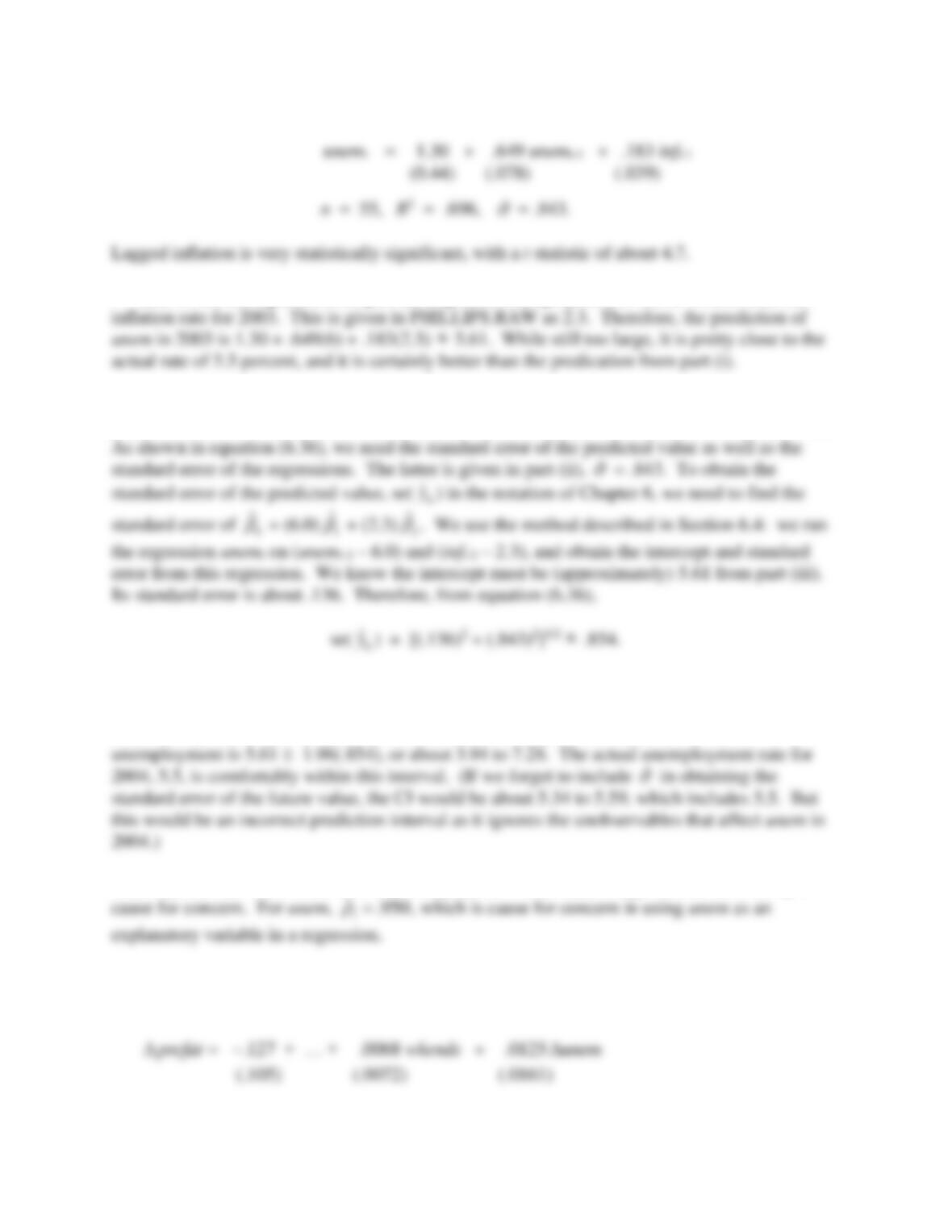
139
(iii) To use the equation from part (ii) to predict unemployment in 2004, we also need the
(iv) We use the model from part (iii) because inft-1 is very significant. To use the 95%
prediction interval from Section 6.4, we assume that unemt has a conditional normal distribution.
Although the OLS estimators are only approximately normally distributed in the presence of a
lagged dependent variable, we use the 97.5th percentile from the normal distribution, 1.96, in
constructing the confidence interval. Therefore, the 95% prediction interval for 2004
C11.9 (i) The first order autocorrelation for prcfat is .709, which is high but not necessarily a
(ii) If we use the first differences of prcfat and unem, but leave all other variables in their
original form, we get the following:
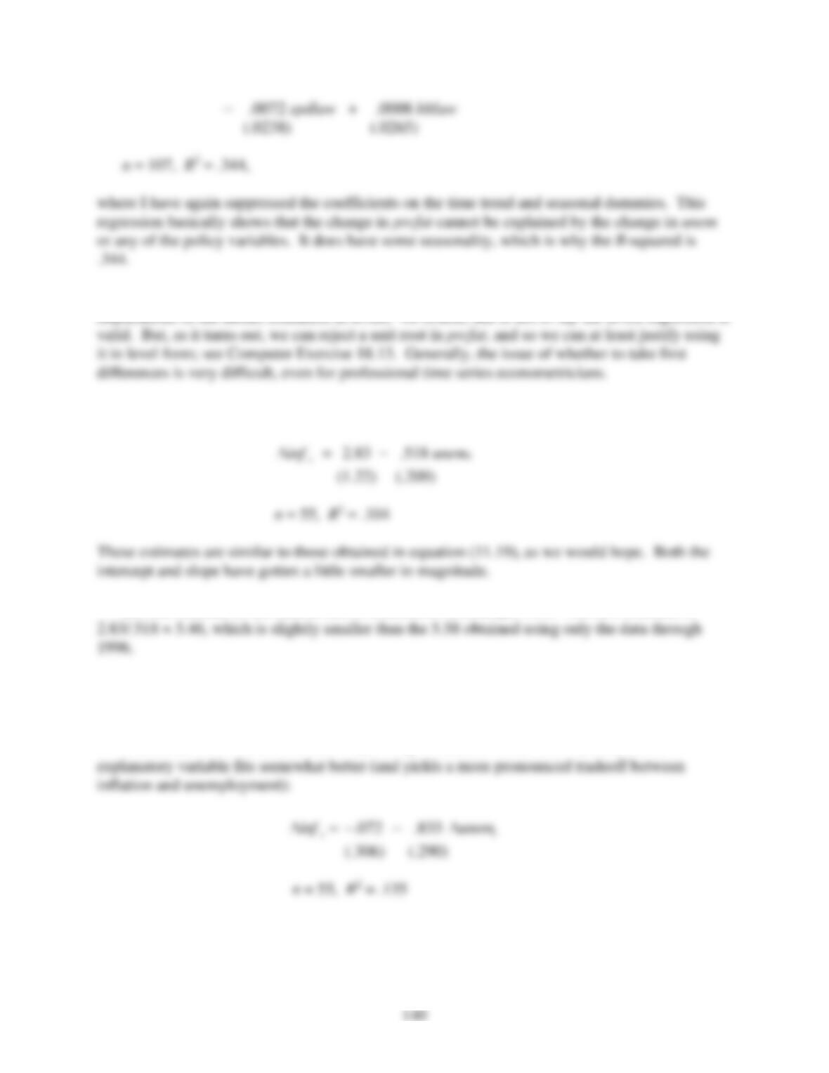
(iii) This is an example about how estimation in first differences loses the interesting
implications of the model estimated in levels. Of course, this is not to say the levels regression is
C11.10 (i) Using the data through 2003 gives
(ii) The estimate of the natural rate is obtained as in Example 11.5. The new estimate is
(iii) The first order autocorrelation of unem is about .75. This is one of those tough cases:
the correlation between unemt and unemt-1 is large, but it is not especially close to one.
(iv) Just as when we use the data only through 1996, the model with
t
unem
t
unem
as the
C11.11 (i) The estimated equation is
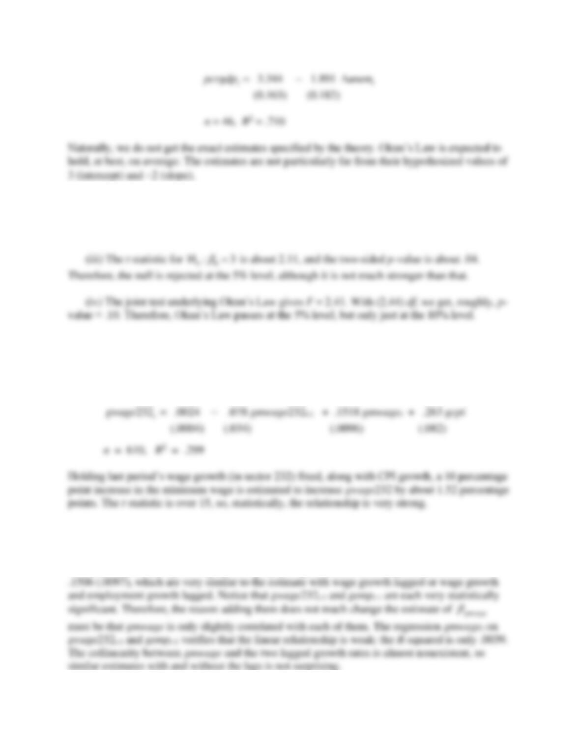
141
(ii) The t statistic for testing
01
H : 2
=−
is about .60, which gives a two-sided p-value of
about .55. This is very little evidence against H0; the null is not rejected at any reasonable
significance level.
C11.12 (i) The first order autocorrelation in gmwage232 is only about −.035, which is very
small. There is little doubt that gmwage232 is I(0) (weakly dependent).
(ii) The estimated equation is
(iii) When gemp232t-1 is added to the regression, the coefficient (standard error) on gmwage
are .1527 (.0095), which is very similar to the estimate and standard error from part (ii).
(iv) Without the lags of wage and employment growth, the estimate (standard error) are
142
C11.13 (i) Rounded to three decimal places, the correlation between urate and uratet-1 is .996,
which is very close to unity. This is indicative of a unit root process.
The relationship is negative and the slope is very statistically significant with |t| > 18.
(iv) Unfortunately, because uratet and vratet cannot be assumed to be weakly dependent, we
(v) The equation estimated in first differences is