1
CHAPTER 11
Monopoly
A. Summary
The traditional theory of monopoly behavior is surveyed in Chapter 11. The
implications of monopolists’ market power for the allocation of resources are
stressed: the deadweight loss of reduced output and the redistribution of sur-
plus from consumers to the firm.
Two extensions of monopoly theory are analyzed in the chapter: price
discrimination and regulation of monopoly. The price discrimination section
distinguishes between two forms: discriminating by separating different
raised by marginal cost pricing for a firm with declining average costs. The
“natural monopoly dilemma” is illustrated and a few solutions are examined.
B. Lecture and Discussion Suggestions
A theoretical lecture on Chapter 11 should make clear why monopolies and
perfectly competitive industries behave differently. One way to make that
Another way to show the difference between monopoly and perfect com-
petition is to contrast the comparative statics analysis of the response to a
shift in demand. Problems 11.3 and 11.4 provide illustrations (perhaps to the
point of tedium) of such shifts that show why the monopoly situation is more
Chapter 11: Monopoly
2
The theory of regulation offers a number of empirical topics that can pro–
vide interesting material for both lectures and discussion based on Chapter 11.
The natural monopoly pricing dilemma can be succinctly covered by reviewing
Figure 11.8. Once this is done, the instructor can raise the discussion point that
C. Glossary Entries in the Chapter
• Barriers to Entry
• Monopoly Rents
SOLUTIONS TO CHAPTER 11 PROBLEMS
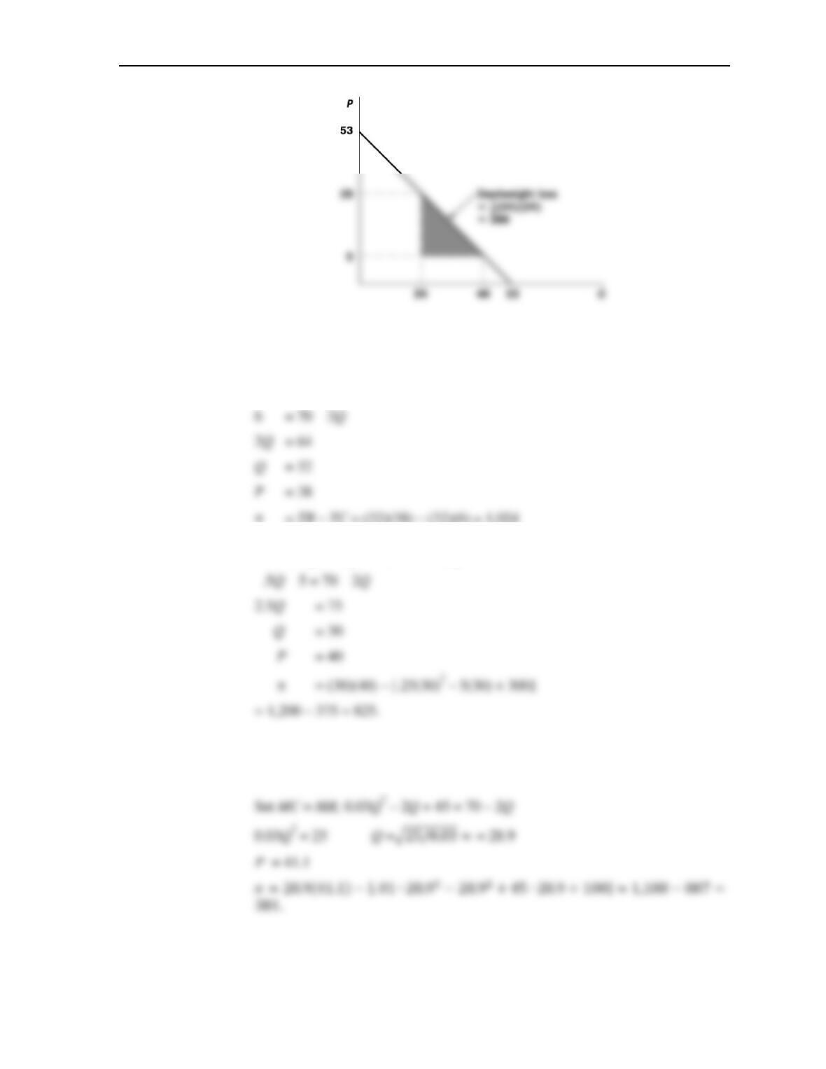
11.1 a. P = 53 – Q.
For maximum profits, set MR = MC:
b. MC = P = 5, P = 5, Q = 48.
Chapter 11: Monopoly
3
11.2 Market Demand Q = 70 – P, MR = 70 – 2Q.
a. AC = MC = 6. To maximize profits set MC = MR.
= TR – TC = (32)(38) – (32)(6) = 1,024
b. TC = .25Q2 – 5Q + 300, MC = .5Q – 5. Set MC = MR
c. TC = 0.01Q3 – Q2 + 45Q +100.
MC = 0.03Q2 – 2Q + 45.
Chapter 11: Monopoly
4
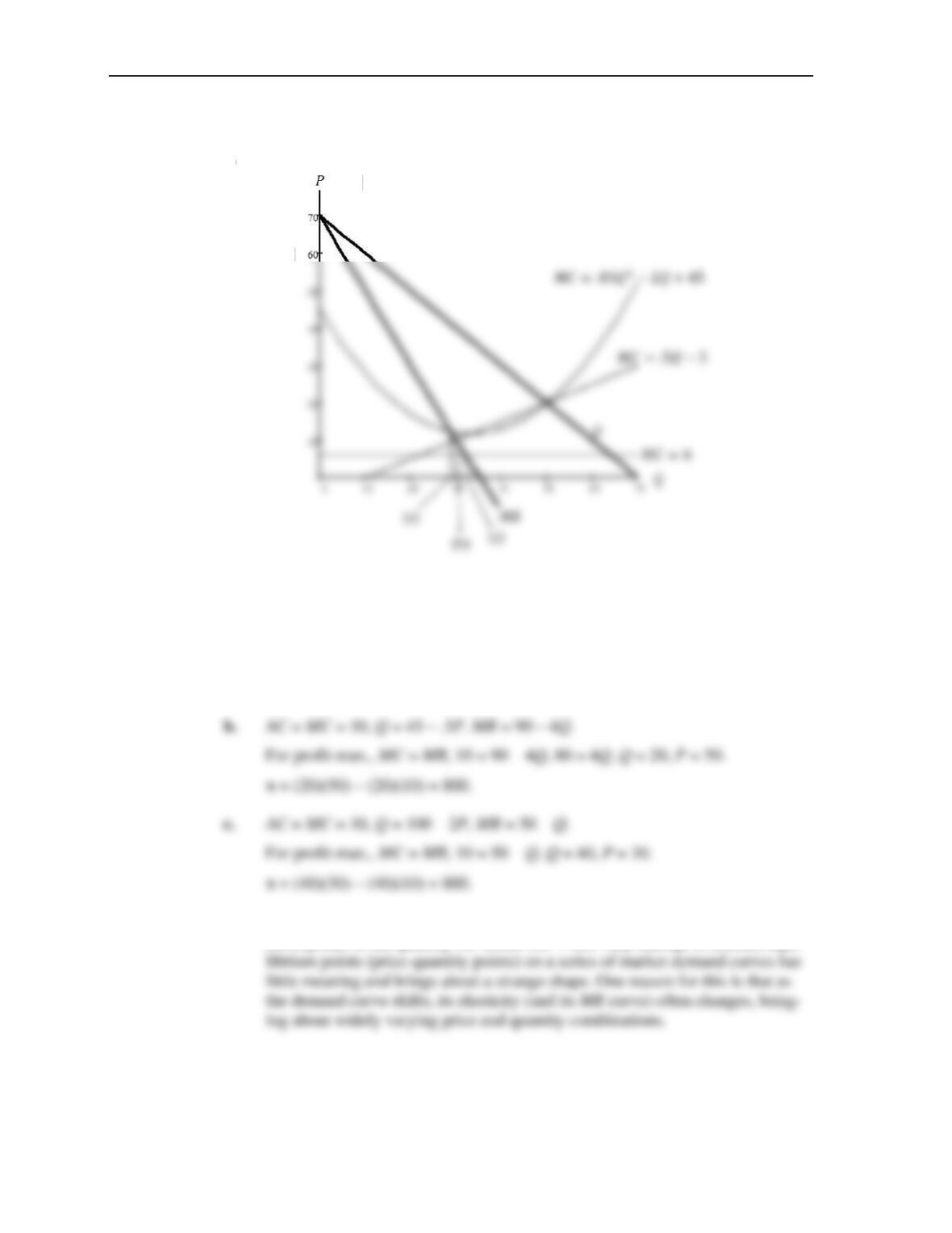
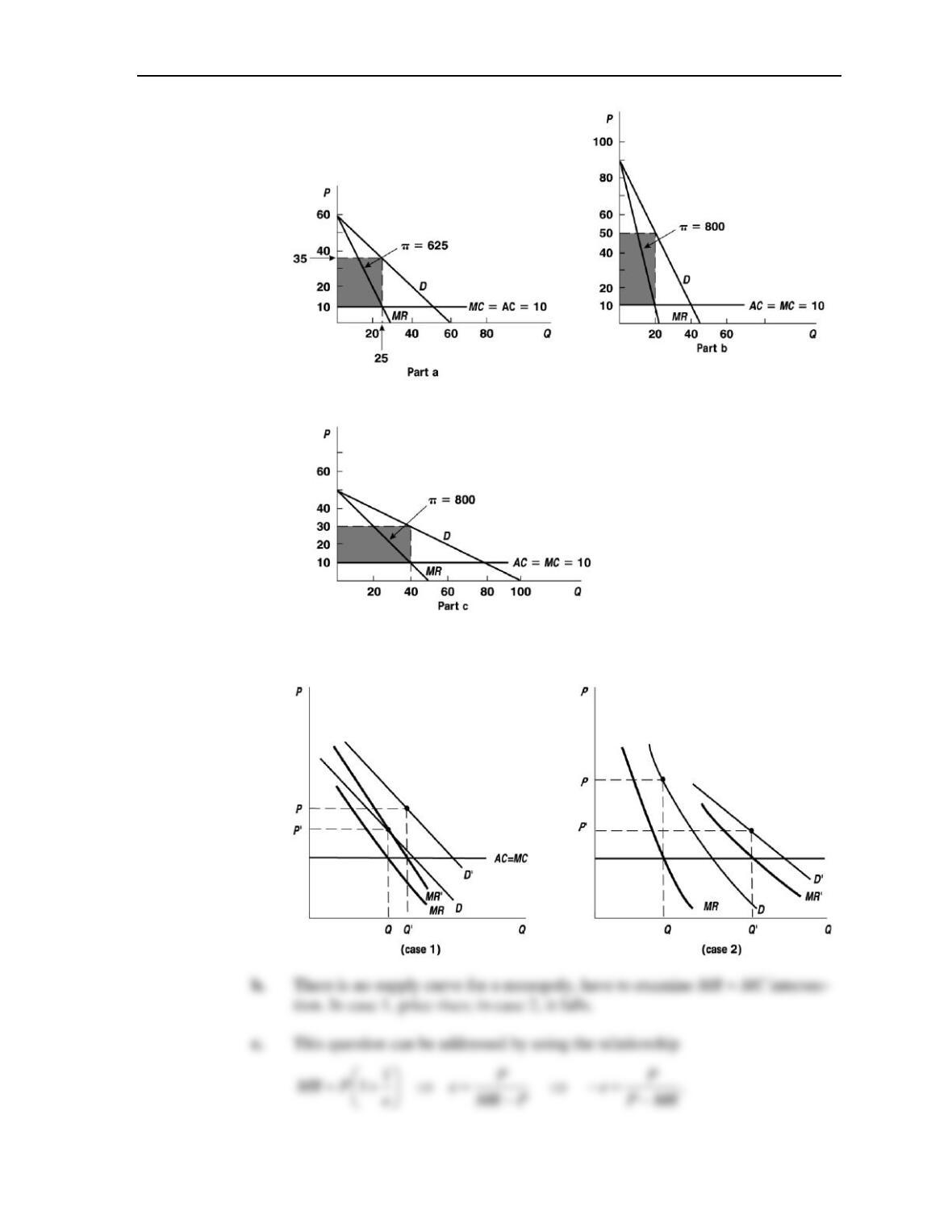
d. The graph shows the solutions to parts a, b, and c. Notice only cost conditions
vary among these three solutions.
11.3 a. AC = MC = 10, Q = 60 – P, MR = 60 – 2Q.
For profit max., MC = MR. 10 = 60 – 2Q, 2Q = 50, Q = 25, P = 35.
= TR – TC = (25)(35) – (25)(10) = 625.
d. The supply curve for a monopoly is the single point on the demand curve that
corresponds to the quantity for which MC = MR. Any attempt to connect equi-
Chapter 11: Monopoly
5
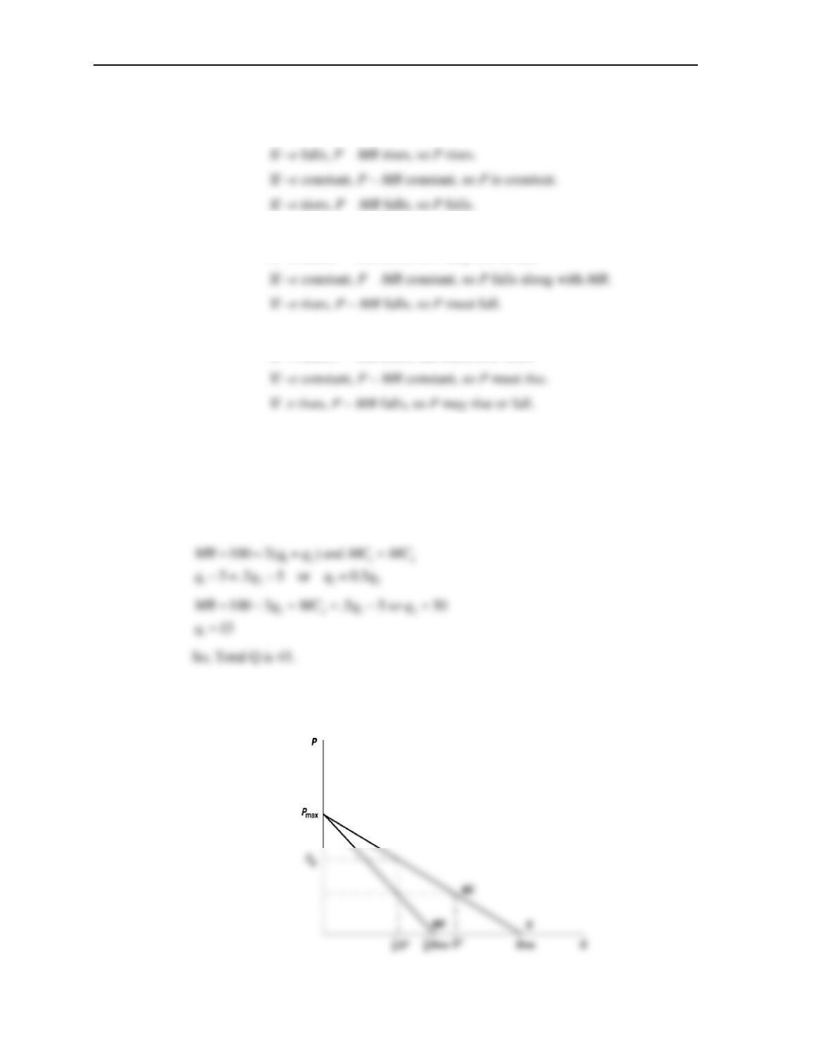
11.4 a. Graph shows shifts in demand (and MR) for two types of shift.
Chapter 11: Monopoly
6
Can use this to study the three cases.
• Case 1 MC constant, so MR is constant.
• Case 2 MC falling, so MR falls as Q expands.
If –e falls, P – MR rises, so P may rise or fall.
• Case 3 MC rising so MR must rise with increases in Q.
If –e falls, P – MR rises, MR rises, so P rises.
This shows P may change in a variety of ways in response to an increase in
demand depending on how elasticity changes.
11.5 A multiplant monopolist will still produce where MR = MC and will equalize MC
among factories.
11.6 a. First prove the hint:
Chapter 11: Monopoly
7
In the graph Qmax is the quantity demanded when P = 0. Since MR = 0 at 1/2Qmax
Note: The results of this hint are used to solve several problems in later chap-
ters.
b. If Q1 = 55 – P, then since MC = 5, Q1 = 55 – 5 = 50
1*
= 25
2
Q
At that output level, P1 = 30
c. This is a hard problem, so let’s work up to the solution in steps. Total profits
The first two equations are self-explanatory. The next step substitutes in the
Chapter 11: Monopoly
8
This is a hump-shaped parabola. You can find its maximum in several ways.
If you know calculus, you can use standard maximization procedures. If you
don’t know calculus, you can use the standard formula for the vertex:
Substituting into the relevant formulas gives 𝑃2
∗=221
3, 𝑄1
∗=312
3, 𝑄2
∗=251
3,
𝜋1
∗=603.2, 𝜋2
∗=439.1, Π∗= 1,042.3.
When the arbitrage cost is $0 between the markets, the prices have to be the
same. Substituting 𝑃2= 𝑃1 into the first set of equations gives
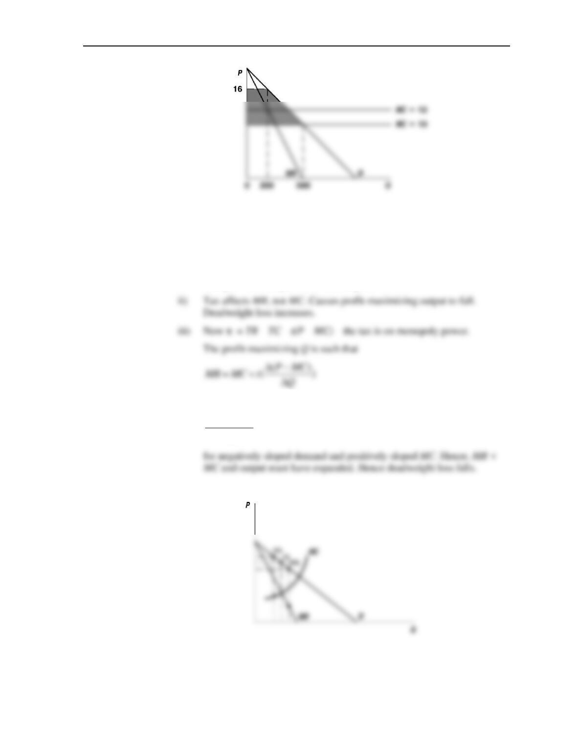
11.7 QD = 1,000 – 50P MR = 20 – Q/25
MC = 10 under PC MC = 12 under monopoly.
a. Perfect competition:
P = MC = 10
b. Loss of consumer surplus due to monopolization can easily be obtained from
the graph (shaded portion).
c. The graph shows that the loss of consumer surplus is much greater here than in
the usual case where monopolization does not affect costs.
Chapter 11: Monopoly
9
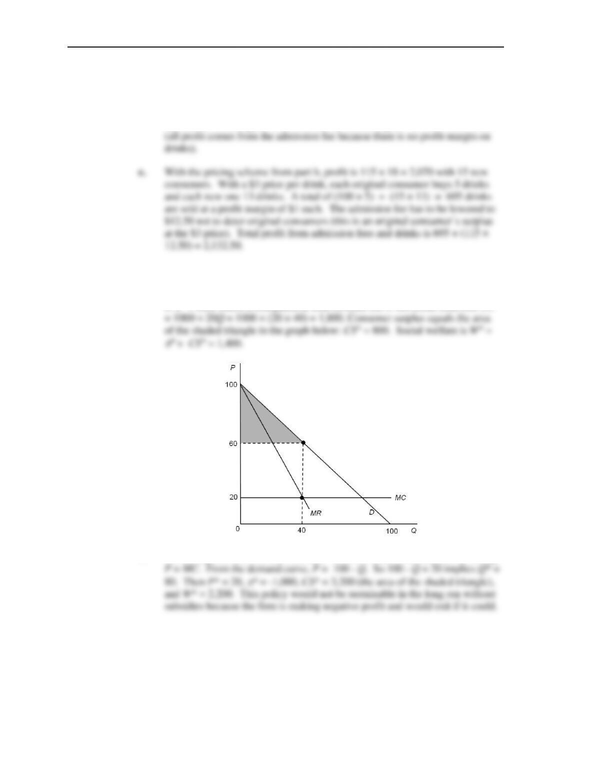
11.8 Result depends on how tax affects MR = MC solution.
a. i) Tax affects MR, MC equally. So profit-maximizing output is not
changed. Deadweight loss is unchanged.
but
()
0
P MC
Q
−
b. The graph shows the three post-tax equilibria:
Chapter 11: Monopoly
10
11.9 a. Setting MR = MC yields Q* = 3. Thus P* = 5 and profit is 9. The profit from
100 such consumers is 900.
b. An individual’s consumer surplus at a price of 2 is 18, the highest admission
fee that can be charged. With 100 such consumers, profit is 100 × 18 = 1,800
11.10 a. Setting MR = MC yields Qm = 40. Substituting into demand, Pm = 60. Profit
is
m = 600, which is computed as total revenue (60 × 40) minus total cost TC
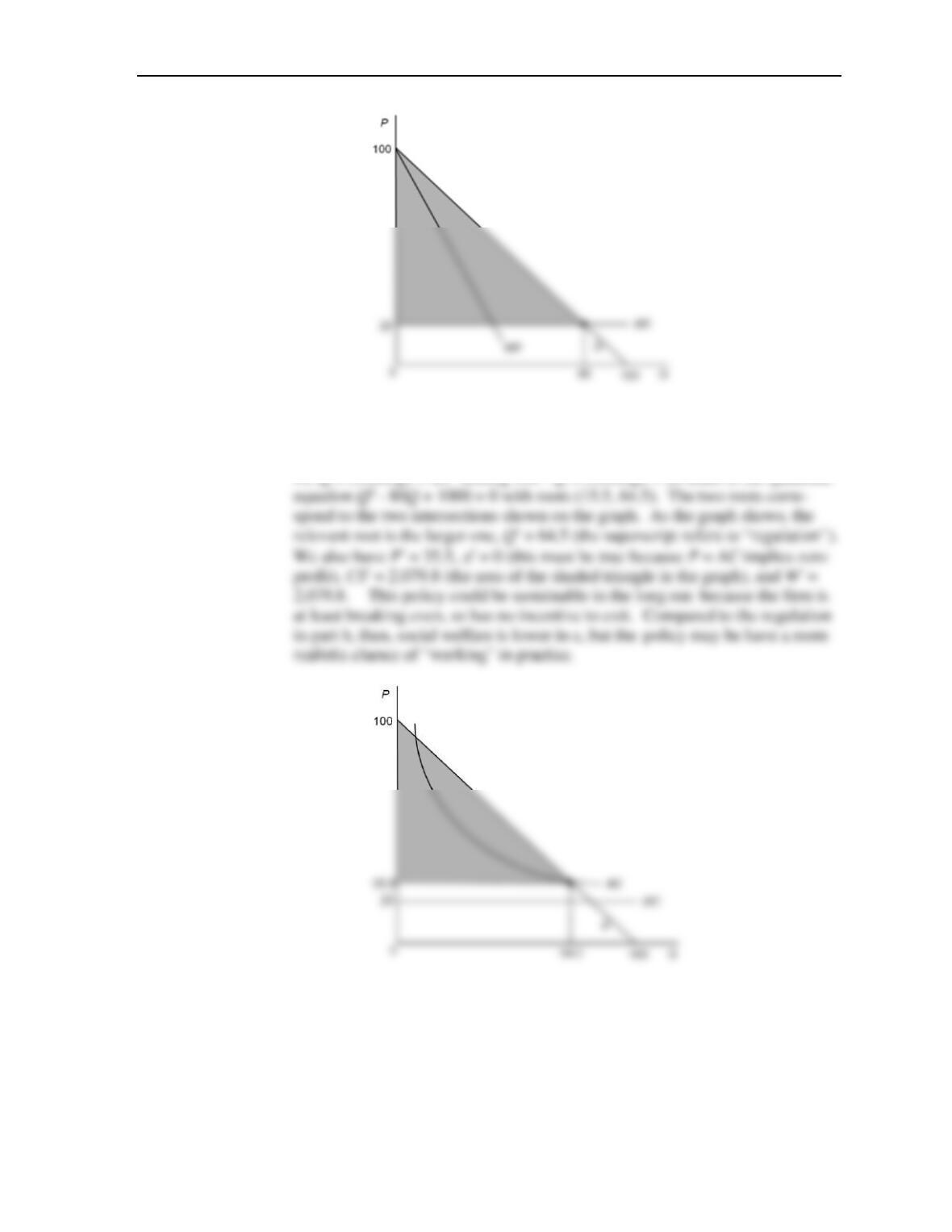
b. See the figure below for this outcome. Social welfare is maximized by setting
Chapter 11: Monopoly
11
c. See the figure below for this outcome. Compute the quantity under this form
of regulation by finding the intersection between P (from the inverse demand
curve) and AC. To compute AC, start from TC = 1000 + 20Q, implying AC =
TC/Q = (1000/Q) + 20. Setting 100 – Q = (1000/Q) + 20 leads to the quadratic