
Chapter 11 Keynesianism: The Macroeconomics of Wage and Price Rigidity 255
7. In response to a recession, policymakers can (1) make no change in macroeconomic policy,
(2) increase the money supply, or (3) increase government purchases.
If they make no change in macroeconomic policy, then during the recession output is below its
full-employment level. Over time, the price level will decline to restore equilibrium. In the long run,
the price level will be lower and employment will return to the full-employment level.
8. Employment is procyclical because a contractionary aggregate demand shock reduces both output
and employment. Money is procyclical because price stickiness means that an increase in the money
supply increases output as the aggregate demand curve moves along the flat, short-run, aggregate
interest rate, moving investment in the same direction as the change in output.
9. The Keynesian theory assumes that demand shocks cause most cyclical fluctuations. This means that
during expansions when employment rises, average labor productivity declines, so it is countercyclical.
10. In Keynesian analysis, a supply shock may reduce output in two ways: (1) a reduction in output,
because the supply shock reduces the marginal product of labor, shifting the FE line to the left; and
expansionary policy risks worsening the already-high rate of inflation.
256 Abel/Bernanke/Croushore • Macroeconomics, Ninth Edition
Numerical Problems
1. The following table shows the real wage (w), the effort level (E), and the effort per unit of real wages
(E/w).
w
E
E/w
8
7
0.875
10
10
1.00
12
15
1.25
14
17
1.21
16
19
1.19
2. (a) The IS curve is found from the equation Y = Cd + Id + G = 130 + 0.5(Y − 100) − 500r + 100 −
500r + 100, or 0.5Y = 280 − 1000r, or Y = 560 − 2000r.
The LM curve comes from the equation M/P = L, which in this case is 1320/P = 0.5Y − 1000r,
Chapter 11 Keynesianism: The Macroeconomics of Wage and Price Rigidity 257
3. (a) Y = C + I + G = [388 + 0.4(Y − 300) − 600r] + [352 − 400r] + 280 = 900 + 0.4Y − 1000r,
so 0.6Y = 900 − 1000r. Therefore, Y = 1500 − (1666 + 2/3)r. Equivalently, r = 0.9 − 0.0006Y.
(b) 12600/7 = M/P = L = 1750 + 0.75Y − 8750(r + 0.02), so 1800 = 1750 + 0.75Y − 8750r − 175.
(d) In long-run equilibrium, output equals its full-employment level, so Y = 1400.
Substitute Y = 1400 into the IS curve to obtain r = 0.9 − 0.0006Y = 0.9 − (0.0006 1400), so r =
0.06.
Consumption = C = 388 + 0.4(Y − T) − 600r = 388 + 0.4(1400 − 300) − (600 0.06), so C = 792.
Investment = I = 352 − 400r = 352 − (400 0.06), so I = 328.
258 Abel/Bernanke/Croushore • Macroeconomics, Ninth Edition
(f) (1) Set I = 320 in the investment equation (I = 352 − 400r) to obtain 320 = 352 − 400r, which
implies 400r = 32. Therefore, the real interest rate must be r = 0.08 to attain I = 320.
(2) In long-run equilibrium, output equals its full-employment level, so Y = 1400. Therefore,
4. (a) The IS curve is given by Y = Cd + Id + G = 300 + 0.5(Y − 100) − 300r + 100 − 100r + 100 = 450
+ 0.5Y − 400r. This can be rewritten as 0.5Y = 450 − 400r, or Y = 900 − 800r. The LM curve is
M/P = L, or 6300/P = 0.5Y − 200r.
5. (a) Setting w = MPN,
10/ .wN=
This is the labor demand curve.
(b) At W = 20, w = W/P = 20/P. Since labor demand is given by
10/ ,wN=
then
20/ 10/ ,PN=
or 2
N
= P.
N
Chapter 11 Keynesianism: The Macroeconomics of Wage and Price Rigidity 259
(d) The IS curve is Y = 120 − 500r. The LM curve is M/P = 0.5Y − 500r, which can be rewritten as
500r = 0.5Y − (M/P). Plugging the LM curve into the IS curve to eliminate r gives Y = 120 −
(f) When the money supply falls to 135, the AD curve becomes 1.5Y = 120 + (135/P), or Y = 80 +
(90/P). The AD curve intersects the SRAS curve where 10P = 80 + (90/P). This can be rewritten
6. (a) Y = Cd + Id + G = [325 + 0.5(1000 − 150) − 500r] + [200 − 500r] + 150, so 1000r = 100,
so r = 0.10.
M/P
=
L, so 6000/P = 0.5Y − 1000r = (0.5 1000) − (1000 0.10) = 400, so P = 15.
(c) Since P = 15 at full employment, then Y = 1000 and r = 0.10.
(d)
IS = (c0 + i0 + G − cYt0)/(cr + ir) = [325 + 200 + 250 − (0.5 150)]/(500 + 500) = 0.7.
260 Abel/Bernanke/Croushore • Macroeconomics, Ninth Edition
Analytical Problems
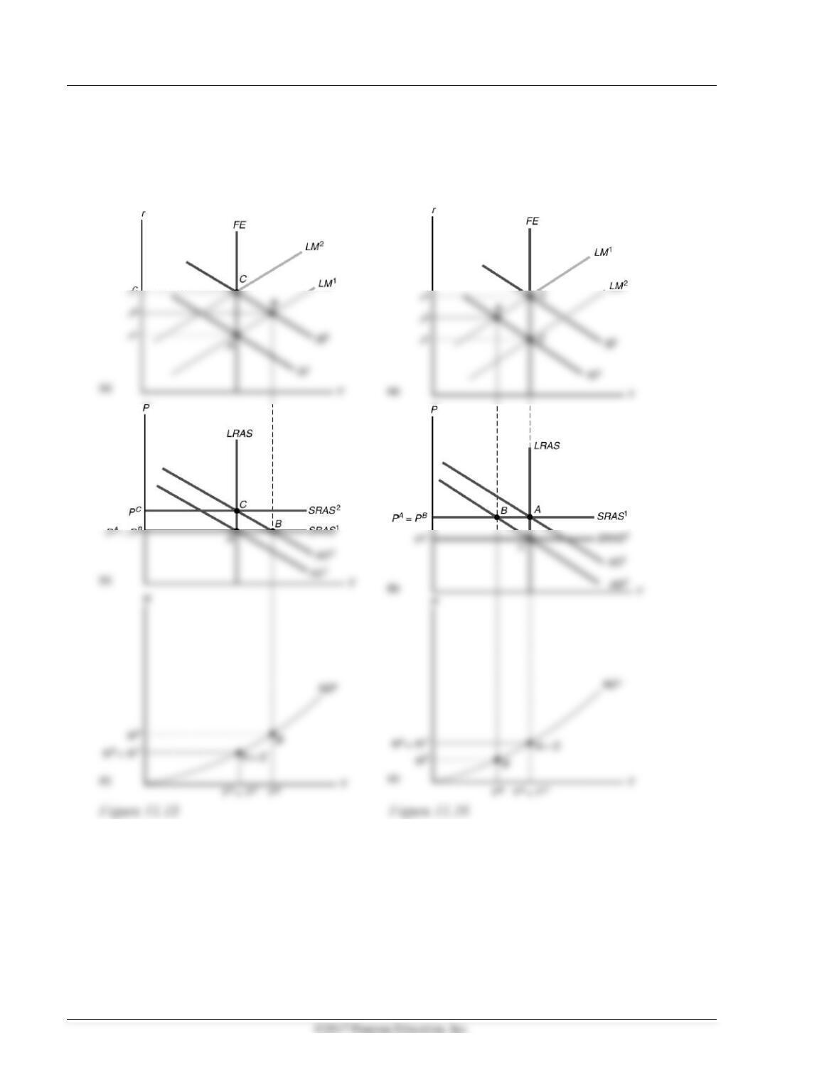
1. In Figures 11.15 and 11.16, point A is the starting point, point B shows the short-run equilibrium after
the change, and point C shows the long-run equilibrium after the change.

Chapter 11 Keynesianism: The Macroeconomics of Wage and Price Rigidity 261
(a) In Figure 11.15, the increase in tax incentives increases investment, shifting the IS curve up and
to the right from IS1 to IS2 in Figure 11.15(a), and shifting the AD curve from AD1 to AD2 in
Figure 11.15(b). The short-run equilibrium is at point B. Output increases, the real interest rate
(b) In Figure 11.16, the increase in tax incentives increases saving—shifting the IS curve from IS1 to
IS2 in Figure 11.16(a), and shifting the AD curve from AD1 to AD2 in Figure 11.16(b). The short-
run equilibrium is at point B. Output decreases, the real interest rate decreases, employment
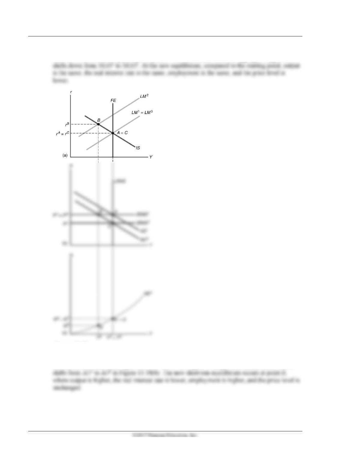
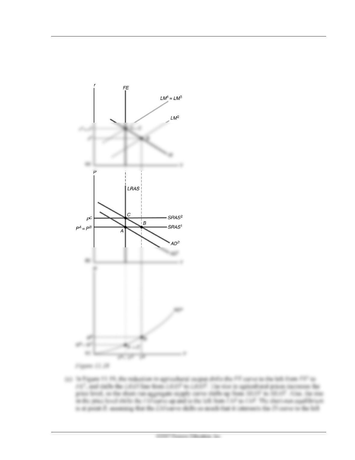
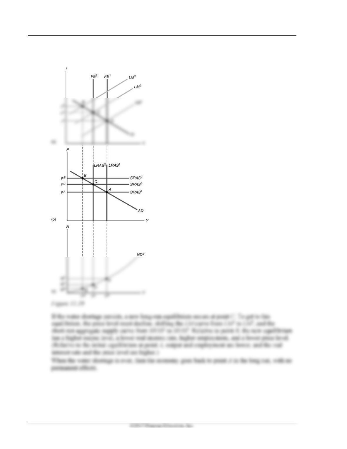
2. In Figures 11.17–11.20, point A is the starting point, point B shows the short-run equilibrium after
the change, and point C shows the long-run equilibrium after the change.
(a) In Figure 11.17, when banks pay a higher interest rate on checking accounts, the demand for
262 Abel/Bernanke/Croushore • Macroeconomics, Ninth Edition
In the long run, the price level decreases to shift the LM curve from LM2 to LM3, which is the
same as LM1, to restore equilibrium at point C. As a result, the short-run aggregate supply curve
Figure 11.17
(b) In Figure 11.18, the introduction of credit cards reduces the demand for money—shifting the
LM curve down and to the right from LM1 to LM2 in Figure 11.18(a). As a result, the AD curve
Chapter 11 Keynesianism: The Macroeconomics of Wage and Price Rigidity 263
In the long run, the price level increases to shift the LM curve from LM2 to LM3, which is the
same as LM1, to restore equilibrium at point C. As a result, the short-run aggregate supply curve
shifts up from SRAS1 to SRAS2. At the new equilibrium, compared to the starting point, output is
the same, the real interest rate is the same, employment is the same, and the price level is higher.
264 Abel/Bernanke/Croushore • Macroeconomics, Ninth Edition
of the FE line. At point B, compared to the starting point, output is lower, the real interest rate is
higher, employment is lower, and the price level is higher.
Chapter 11 Keynesianism: The Macroeconomics of Wage and Price Rigidity 265
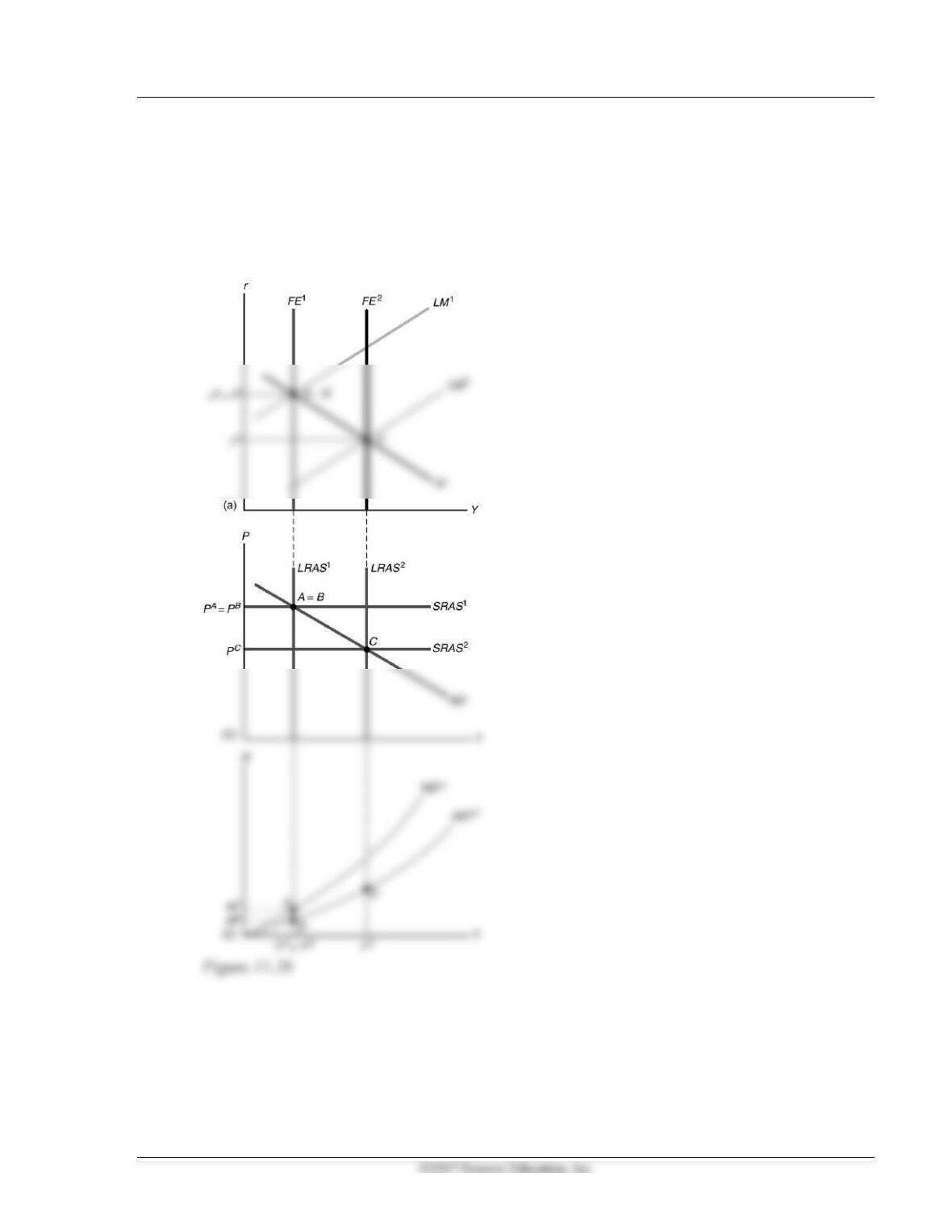
(d) In Figure 11.20, the beneficial supply shock makes more production possible at full employment,
so the FE line shifts to the right in Figure 11.20(a) from FE1 to FE2, and the LRAS line shifts from
LRAS1 to LRAS2 in Figure 11.20(b). There is no immediate change in the price level, so the LM
curve remains at LM1 and the short-run aggregate supply curve remains at SRAS1. The shift of
the FE curve does not affect aggregate demand in the short run: output, the real interest rate, and
the price level are all unchanged in the short run. The shift in the production function shifts the
effective labor demand curve and reduces employment in the short run.
If the supply shock persists, prices will decline, so the LM curve will shift from LM1 to LM2 and
the SRAS curve will shift from SRAS1 to SRAS2. As shown in the diagrams, the economy reaches
a new equilibrium at point C, with a higher output level, a lower real interest rate, and a lower
price level.
When the supply shock disappears, the economy returns to its equilibrium at point A.
266 Abel/Bernanke/Croushore • Macroeconomics, Ninth Edition
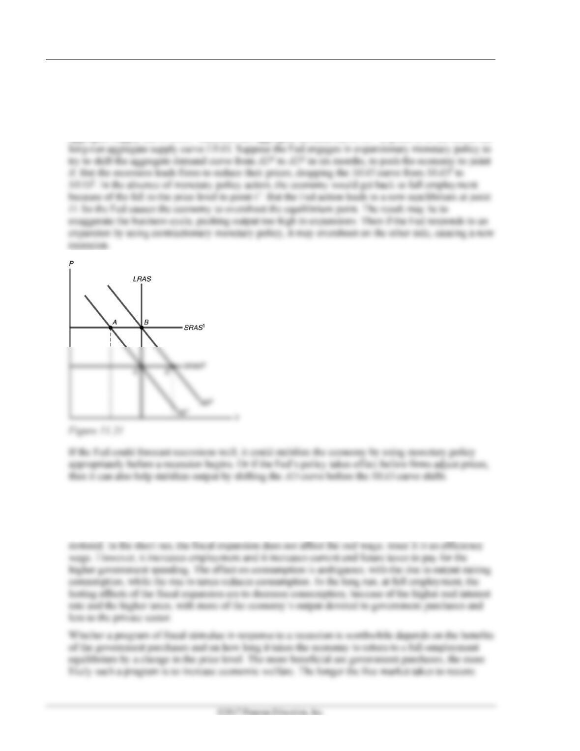
3. A lag in the impact of policy of six months, which is about the time it takes firms to adjust prices,
could cause policy to be destabilizing. That is, monetary policy may be pushing the economy away
from equilibrium.
To see this, suppose the economy is in a recession at point A in Figure 11.21. The short-run
aggregate-supply curve SRAS1 intersects the aggregate demand curve AD1 at point A, to the left of the
4. An increase in government purchases shifts the IS curve up and to the right and the AD curve up and
to the right to return the economy to full employment, instead of waiting for the price level to fall to
get there. The advantage of doing so, according to Keynesians, is that full employment is restored
quickly, whereas if the price level must adjust, it may take a long time for full employment to be

Chapter 11 Keynesianism: The Macroeconomics of Wage and Price Rigidity 267
268 Abel/Bernanke/Croushore • Macroeconomics, Ninth Edition
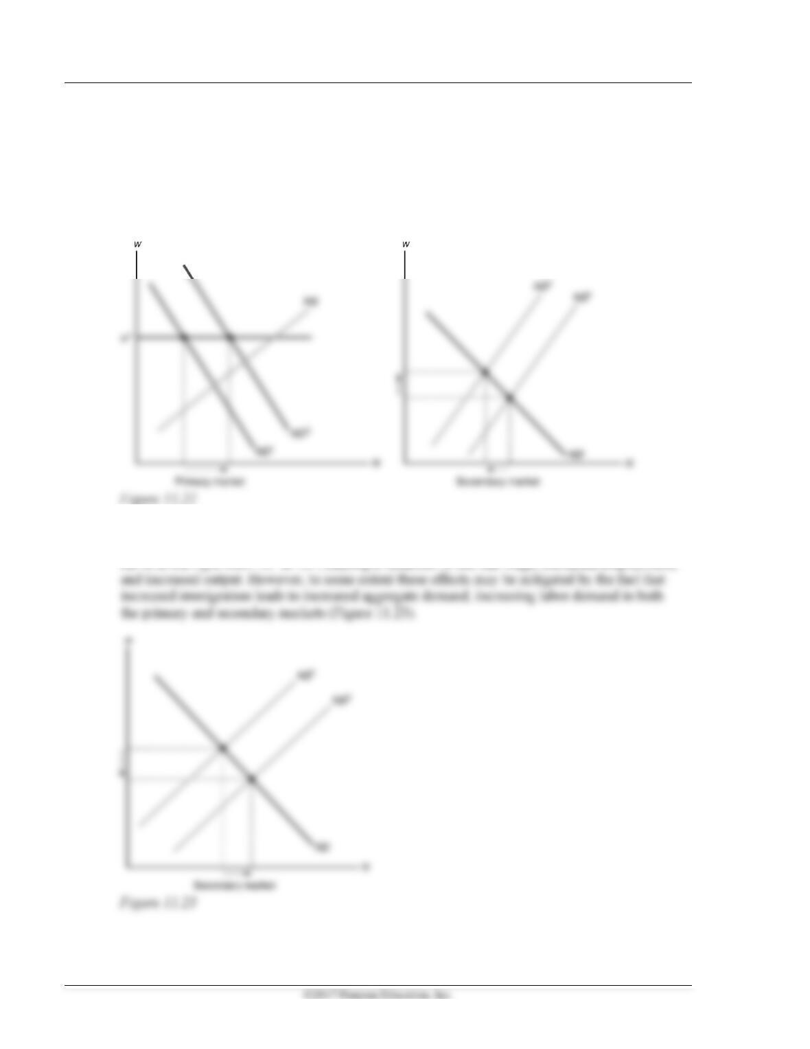
5. (a) In response to expansionary monetary policy, aggregate demand increases, increasing output and
labor demand. This causes the labor demand curve to shift from ND1 to ND2 in the primary labor
market, shown in Figure 11.22. The result is an increase in employment and output with no
change in the real wage in the primary labor market. Since more workers are now in the primary
labor market, the labor supply in the secondary labor market decreases from NS1 to NS2. This causes
an increase in the real wage, a decrease in employment, and a decrease in output in the secondary
labor market.
(b) Increased immigration has no effect in the primary labor market, since labor supply changes in
general have no effect. In the secondary labor market, the immigration shifts the labor supply
curve to the right from NS1 to NS2, causing a reduction in the real wage, increased employment,
Chapter 11 Keynesianism: The Macroeconomics of Wage and Price Rigidity 269
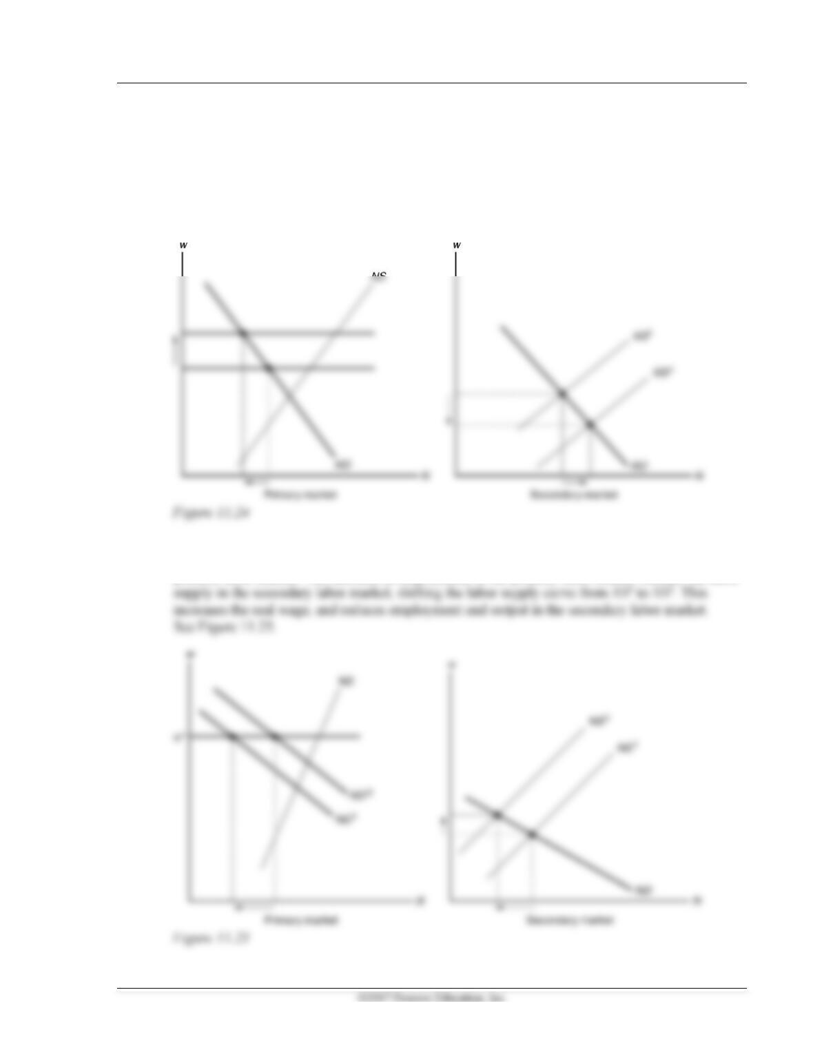
(c) If there is a shift in the effort curve, the efficiency wage rises in the primary labor market. Since
effort exerted at the higher wage is the same as before the change, the shift in the effort curve has
no impact on the marginal product of labor, so there is no shift in the labor demand curve. So the
effect of the higher real (efficiency) wage is to reduce employment and thus output in the primary
labor market. This means that labor supply in the secondary labor market increases, shifting the
labor supply curve from NS1 to NS2. The real wage falls, employment rises, and output rises in
the secondary labor market, as Figure 11.24 shows.
(d) The productivity improvement shifts the labor demand curve to the right, so at the fixed real
(efficiency) wage, firms demand more labor. Employment increases, so output increases in the
primary labor market. The increase in employment in the primary labor market reduces the labor
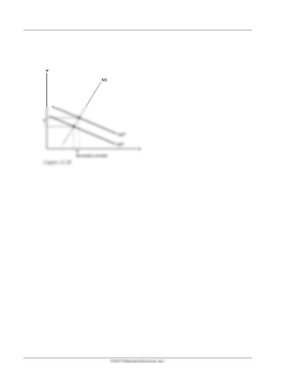
270 Abel/Bernanke/Croushore • Macroeconomics, Ninth Edition
(e) The productivity improvement in the secondary labor market has no effect on the primary labor
market. In the secondary labor market, increased productivity increases the marginal product of
labor so that labor demand increases from ND1 to ND2. The result is a higher real wage, higher
employment, and increased output (Figure 11.26).

Chapter 11 Keynesianism: The Macroeconomics of Wage and Price Rigidity 271
Working with Macroeconomic Data
1. In the 1980s, usually the federal government deficit/GDP moved in the opposite direction as the
short-term real interest rate and in the 2000s the federal government deficit/GDP moved in the
2. Between 1960 and 1980, an increase in the money growth rate is followed after several years by
3. Classical economists would argue that the supply shock was the sole cause of the recession. But