
CHAPTER 11: CLASSICAL BUSINESS CYCLE ANALYSIS:
MARKET–CLEARING MACROECONOMICS
LEARNING OBJECTIVES
I. Goals of Chapter 11
A. Use the IS-LM/AD-AS model with rapidly adjusting wages and prices to
TEACHING NOTES
I. Business Cycles in the Classical Model (Sec. 11.1)
A. The real business cycle theory
1. Any business cycle theory has two components
a. A description of the types of shocks believed to affect the
2. Real business cycle (RBC) theory
a. Real shocks to the economy are the primary cause of business
cycles
(1) Examples: Shocks to the production function, the size of
b. The largest role is played by shocks to the production function,
which the text has called supply shocks, and RBC theorists call
productivity shocks
(1) Examples: Development of new products or production
methods, introduction of new management techniques,
changes in the quality of capital or labour, changes in the
196 Chapter 11
causes a boom (output increases); but output always
equals full-employment output
d. Real business cycle theory and the business cycle facts
(1) The RBC theory is consistent with many business cycle
facts
and real wages
Numerical Problem 1 looks at the relationship between real wages and employment
over the business cycle and the issue of whether the labour-supply curve should be flat
or steep to be consistent with the data.
(c) The theory correctly predicts procyclical average
labour productivity, if booms weren’t due to
(2) The theory predicts countercyclical movement of the price
level, which seems to be inconsistent with the data
(a) But R. Todd Smith, when using some newer statistical
techniques for calculating the trends in inflation and
3. Application: Calibrating the business cycle
a. A major element of RBC theory is that it attempts to make
quantitative, not just qualitative, predictions about the business
Classical Business Cycle Analysis: Market–Clearing Macroeconomics 197
(2) Then they use existing studies of the economy to choose
numbers for parameters like a in the production function;
match post-World War II data fairly well
Data Application
For a good survey article on real business cycles, see George Stadler, “Real Business
Cycles.” Journal of Economic Literature, December 1994, pages 1750–83.
4. Are productivity shocks the only source of recessions?
a. Critics of the RBC theory suggest that except for the oil price
Numerical Problem 5 shows how the growth in Solow residual relates to the growth in
productivity.
Theoretical Application
For more on criticisms of the RBC theory and the RBC response to the critics, see the
discussion in the Federal Reserve Bank of Minneapolis Quarterly Review, Fall 1986,
and the Journal of Economic Perspectives, Summer 1989.
5. Does the Solow residual measure technology shocks?
a. RBC theorists measure productivity shocks as the Solow
residual
(1) Named after Robert Solow, the originator of modern growth
theory

198 Chapter 11
(1) If it’s a measure of technology, it should not be related to
d. Measured productivity can vary even if the actual technology
doesn’t change
(1) Capital and labour are used more intensively at times
(2) More intensive use of inputs leads to higher output
(7) So the Solow residual isn’t just A, but depends on uK and
uN
(8) Utilization is procyclical, so the measured Solow residual is
more procyclical than is the true productivity term A
(a) Burnside-Eichenbaum-Rebelo evidence on procyclical
utilization of capital
e. Conclusion: Changes in the measured Solow residual don’t
necessarily reflect changes in technology
f. Also, the critics suggest that shocks other than productivity
shocks, such as wars and military buildups, have caused
business cycles

Classical Business Cycle Analysis: Market–Clearing Macroeconomics 199
B. Fiscal policy shocks in the classical model
1. The effects of a temporary increase in government expenditures (Fig.
11.1; like text Fig. 11.5)
a. The current or future taxes needed to pay for the government
expenditures effectively reduce people’s wealth, causing an
income effect on labour supply
b. The increased labour supply leads to a fall in the real wage and
a rise in employment
c. The rise in employment increases output, so the FE line shifts to
Analytical Problems 2, 3, and 6 deal with various aspects of the classical IS–LM model.
2. Should fiscal policy be used to dampen the cycle?
a. Classical economists oppose attempts to dampen the cycle,

200 Chapter 11
c. Instead, government spending should be determined by cost-
benefit analysis
d. Also, there may be lags in enacting the correct policy and in
C. Unemployment in the classical model
1. In the classical model there is no unemployment; people who aren’t
working are voluntarily not in the labour force
2. In reality measured unemployment is never zero, and it is the problem
of unemployment in recessions that concerns policymakers the most
3. Classical economists have a more sophisticated version of the model
to account for unemployment
a. Workers and jobs have different requirements, so there is a
matching problem
Theoretical Application
A nice discussion of the classical view of unemployment is by Robert E. Lucas, Jr..
Models of Business Cycles, Chapter V, New York: Basil Blackwell, 1987.
4. A recent study by Balakrishnan of IMF suggests a great deal of
Numerical Problem 6 is a coin-flipping exercise to show that random shocks can lead to
big aggregate movements.
6. But this worker match theory can’t explain all unemployment
a. Many workers are laid off temporarily; there’s no mismatch, just
a change in the timing of work

Classical Business Cycle Analysis: Market–Clearing Macroeconomics 201
the labour market
D. Household production
1. Household production is output produced at home instead of in a
market and therefore is not reflected in the national income accounts
2. Home production includes such goods and services as cooking, child-
II. Money in the Classical Model (Sec. 11.2)
A. Monetary policy and the economy
Money is neutral in both the short run and the long run in the classical model,
because prices adjust rapidly to restore equilibrium
B. Monetary nonneutrality and reverse causation
1. If money is neutral, why do the data show that money is a leading,
procyclical variable?
2. The classical answer: Reverse causation
a. Just because changes in money growth precede changes in
output doesn’t mean that the money changes cause the output
changes
b. Example: People put storm windows on their houses before

202 Chapter 11
Data Application
A recent review of empirical work testing the RBC theory of reverse causation is Shaghil
Ahmed, “Does Money Affect Output?” Federal Reserve Bank of Philadelphia Business
Review, July/August 1993. He finds mixed support for reverse causation, but does
suggest that money growth is unlikely to be a major factor causing business cycles.
3. Why would higher future output cause people to increase money
demand?
a. Firms, anticipating higher sales, would need more money for
Theoretical Application
The early theoretical RBC models did not include a monetary sector at all—they
assumed that money was unimportant for the business cycle. More recently, RBC
theorists have been trying to incorporate money into their models. The focus so far has
been trying to get the models to produce a liquidity effect. in which an increase in the
money supply temporarily reduces nominal interest rates. See, Lawrence J. Christiano,
“Modelling the Liquidity Effect of a Money Shock,” Federal Reserve Bank of Minneapolis
Quarterly Review, Winter 1991.
C. A Closer Look 11.1: Money and economic activity at Christmastime
Analytical Problem 4 works out another example of how reverse causation could occur
through firms’ demand for money for transactions and the central bank’s money-supply
response.
D. The nonneutrality of money: Additional evidence
1. Friedman and Schwartz have extensively documented that often
monetary changes have had an independent origin; they weren’t just a
reflection of changes or future changes in economic activity
a. These independent changes in money supply were followed by

Classical Business Cycle Analysis: Market–Clearing Macroeconomics 203
Theoretical Application
For a thorough overview of how money works to affect the economy in various models,
see the symposium on “The Monetary Transmission Mechanism,” in the Journal of
Economic Perspectives, Fall 1995.
2. Romer and Romer reviewed and updated the Friedman-Schwartz
analysis and found money is not neutral
Numerical Problems 2 and 3 and Analytical Problem 5 examine price level effects in the
classical model.
III. The Misperceptions Theory and the Non-neutrality of Money (Sec. 11.3)
A. Introduction to the misperceptions theory
1. In the classical model, money is neutral since prices adjust quickly
a. In this case, the only relevant supply curve is the long-run
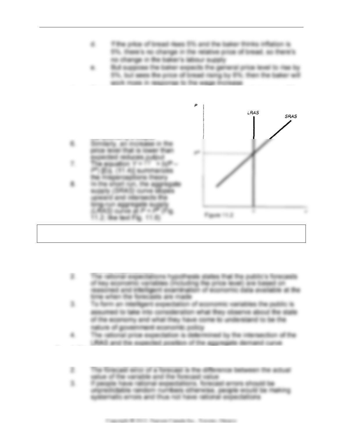
B. The misperceptions theory
1. The misperception theory is that the aggregate quantity of output
supplied rises above the full-employment level Y when the aggregate
price level P is higher than expected
2. This makes the AS curve slope upward
3. Example: A bakery that makes bread
a. The price of bread is the baker’s nominal wage; the price of
204 Chapter 11
4. Generalizing this example, if everyone expects prices to increase 5%
but they actually increase 8%,
they’ll work more
5. So an increase in the price
level that is higher than
expected induces people to
work more and thus increases
Analytical Problem 1 contrasts the effects of a change in the future marginal product of
capital in an RBC model to that in a misperceptions model.
C. Rational price expectations
1. Economists suggest that it is reasonable to assume that in the face of
uncertainty about the future, the public calculate what is known as
rational expectations
D. A Closer Look 11.2: Are price forecasts rational?
1. Economists can test whether price forecasts are rational by looking at
surveys of people’s expectations

Classical Business Cycle Analysis: Market–Clearing Macroeconomics 205
4. Many statistical studies suggest that people don’t have rational
expectations
5. But people who answer surveys may not have a lot at stake in making
forecasts, so couldn’t be expected to produce rational forecasts
Data Application
The survey used by Keane and Runkle was begun by Victor Zarnowitz of the University
of Chicago in 1968 and was run by the American Statistical Association and National
Bureau of Economic Research until 1990. At that time the survey was taken over by the
Federal Reserve Bank of Philadelphia and christened the “Survey of Professional
Forecasters.” See the article by Dean Croushore, “Introducing: The Survey of
Professional Forecasters,” Federal Reserve Bank of Philadelphia Business Review,
November/December 1993. Unfortunately, there is nothing comparable here in Canada.
E. Monetary policy and the misperceptions theory
1. Because of misperceptions,
unanticipated monetary policy
2. Unanticipated changes in the
money supply (Fig. 11.3; like text
Fig. 11.9)
a. Initial equilibrium where
AD1 intersects SRAS1 and
LRAS
3. Anticipated changes in the money supply
a. If people anticipate the change in the money supply and thus in
the price level, they aren’t fooled, there are no misperceptions,

206 Chapter 11
F. Rational expectations and the role of monetary policy
1. The only way the central bank can use monetary policy to affect output
is to surprise people
Data Application
Do the data support the misperceptions theory? Robert Barro, “Unanticipated Money,
Output, and the Price Level in the United States,” Journal of Political Economy, August
1978, pp. 549–580, found support for the misperceptions theory; his results suggested
that output was affected only by unanticipated money growth. But others challenged
these results and found that both anticipated and unanticipated money growth seem to
affect output. See Frederic S. Mishkin, “Does Anticipated Monetary Policy Matter? An
4. So even if smoothing the business cycle were desirable, the
G. Propagating the effects of unanticipated changes in the money supply
1. It doesn’t seem that people could be fooled for long, since money
supply figures are reported weekly and inflation is reported monthly
2. Classical economists argue that propagation mechanisms allow short-
lived shocks to have long-lived effects
3. Example of propagation: The behaviour of inventories
a. Firms hold a normal level of inventories against their normal
the economy
IV. Key Diagram 10: The Upward Sloping Short Run Aggregate Supply Curve
A. Diagram Elements
i. The SRAS curve shows the amount of output firms are willing to
offer for sale in the short run and its position is determined by the
expected price level.