Chapter 11
Models for Panel Data
◼ Exercises
1. The pooled least squares estimator is
The fixed effects regression can be computed just by including the three dummy variables since the
sample sizes are quite small. The results are
The F statistic for testing the hypothesis that the constant terms are all the same is
In order to estimate the random effects model, we need some additional parameter estimates.
The group means are
y
x
In the group means regression using these three observations, we obtain
There is only one degree of freedom, so this is the candidate for estimation of
22
/.
u
T
+
In the least
squares dummy variable (fixed effects) regression, we have an estimate of
2
of 79.183/26 = 3.045.
One ought to proceed with some caution at this point, but it is difficult to place much faith in the group
means regression with but a single degree of freedom, so this is probably a preferable estimator in any
Chapter 11 Models for Panel Data 97
For the LM test, we return to the pooled ordinary least squares regression. The necessary quantities
2. There is no effect on the coefficients of the other variables. For the dummy variable coefficients,
with the full set of n dummy variables, each coefficient is
*
y
= mean residual for the ith group in the
3. (a) The pooled OLS estimator will be
1
11
nn
i i i i i i
−
==
=
b X X X y
where Xi and yi have Ti
(b) We seek to establish consistency, not unbiasedness. As such, we will ignore the degrees of freedom
correction, −K, in (11-40). Use n(T − 1) as the denominator. Thus, the question is whether
2
1 1 . 2
()
nT
i t it i
ee
==
− =
98 Greene • Econometric Analysis, Seventh Edition
The second term will converge to zero as the center matrix converges to a constant Q and the
vectors converge to zero as b converges to . (We use the Slutsky theorem.) The third term
4. To find plim(1/n)LM = plim [T/(2(T − 1))]{[i(teit)2]/[iteit2] − 1}2 we can concentrate on the sums
inside the curled brackets. First, i(teit)2 = nT 2{(1/n)i [(1/T)teit]2} and i teit2 = nT(1/(nT))iteit2.
5. The ordinary least squares regression results are
R2 = 0.92803, ee = 146.761, 40 observations.
Variable Coefficient Standard Error
X2 1.83915 0.1534
Constant 3.60568 2.555
Period 1 −3.57906 1.723
Period 6 −1.49474 1.714
Chapter 11 Models for Panel Data 99
Estimated covariance matrix for the slopes:
1 2
1 0.0062209
For testing the hypotheses that the sets of dummy variable coefficients are zero, we will require the
sums of squared residuals from the restrictions. These are
Regression Sum of Squares
All variables included 146.761
The F statistics are therefore,
(1) F[9,25] = [(318.503 − 146.761)/9]/[146.761/25] = 3.251
(3) F[12,25] = [(585.622 − 146.761)/12]/[146.761/25] = 6.23
6. The covariance matrix would be
2 2 2 2 2
1, 1 1, 2 2, 1 2, 2
1, 1 0
u v u v
i t i t i t i t
it
= = = = = = = =
= = + +
7. The two separate regressions are as follows:
Sample 1 Sample 2
b = xy/xx 4/5 = 0.8 6/10 = 0.6
ee = yy − bxy 20 − 4(4/5) = 84/5 10 − 6(6/10) = 64/10
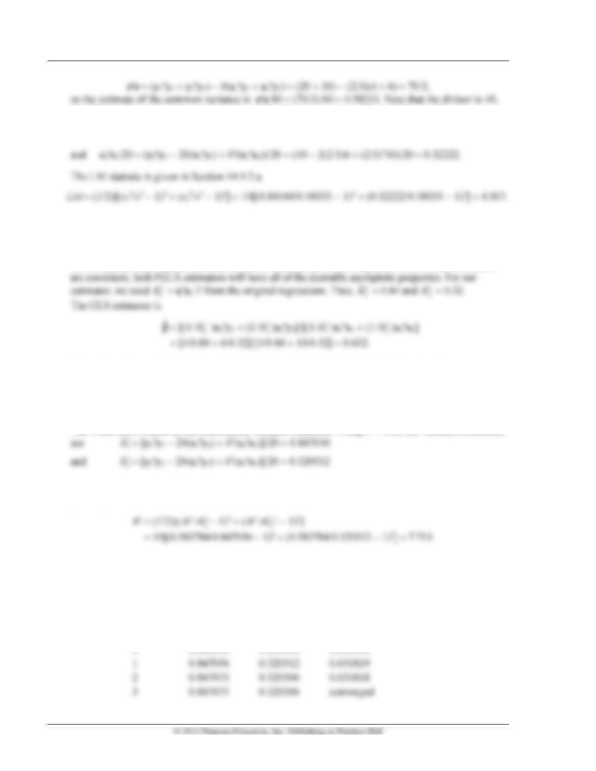
To carry out a Lagrange multiplier test of the hypothesis of equal variances, we require the separate
and common variance estimators based on the restricted slope estimator. This, in turn, is the pooled
least squares estimator. For the combined sample, we obtain
2
ˆ
100 Greene • Econometric Analysis, Seventh Edition
not 39, because we are computing maximum likelihood estimators. The individual estimators are
e1e1/20 = (y1y1 − 2b(x1y1) + b2(x1x1))/20 = (20 − 2(2/3)4 + (2/3)25)/20 = 0.84444
This has one degree of freedom for the single restriction. The critical value from the chi-squared table is
3.84, so we would reject the hypothesis.
In order to compute a two step GLS estimate, we can use either the original variance estimates based
on the separate least squares estimates or those obtained above in doing the LM test. Since both pairs
The estimated sampling variance is 1/[(1/
2
1
ˆ)
x1x1 + (1/
2
2
ˆ
)x2x2] = 0.02688. This implies an
asymptotic standard error of (0.02688)2 = 0.16395. To test the hypothesis that = 1, we would referz =
(0.632 − 1)/ 0.16395 = −2.245 to a standard normal table. This is reasonably large, and at the usual
significance levels, would lead to rejection of the hypothesis.
The Wald test is based on the unrestricted variance estimates. Using b = .632, the variance estimators
while the pooled estimator would be
2
ˆ
= [yy − 2b(xy) + b2(xx)]/40 = 0.583784. The statistic is
given at the end of Example 16.3,
We reach the same conclusion as before.
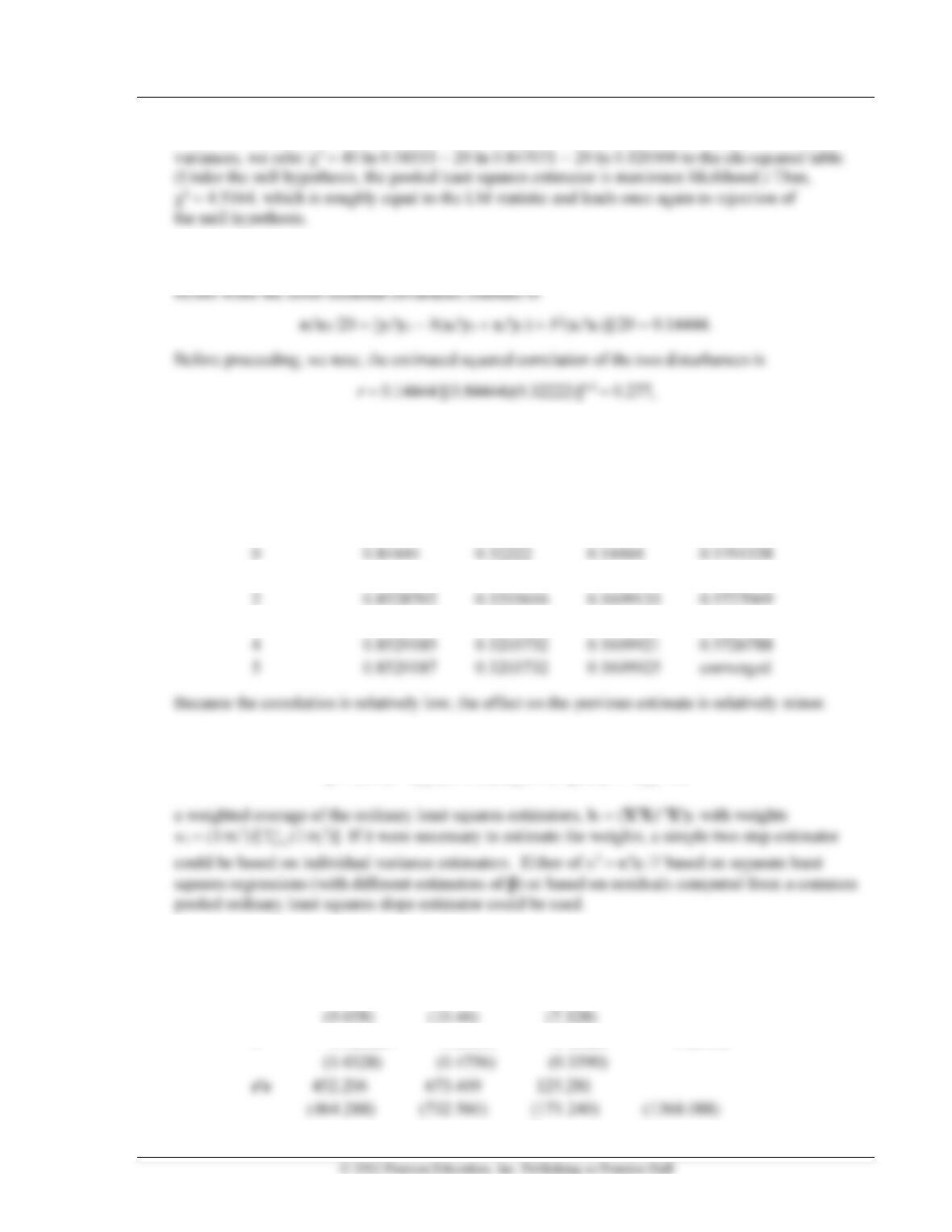
To compute the maximum likelihood estimators, we begin our iterations from the two separate
ordinary least squares estimates of b which produce estimates
2
1
ˆ
= 0.84 and
2
2
ˆ
= 0.32.
The iterations are
Iteration
2
1
ˆ
2
2
ˆ
Chapter 11 Models for Panel Data 101
Now, to compute the likelihood ratio statistic for a likelihood ratio test of the hypothesis of equal
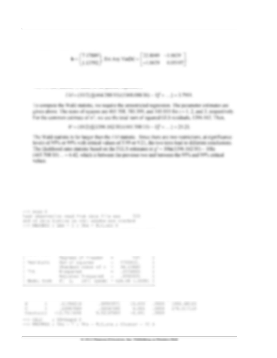
Finally, we allow for cross-sectional correlation of the disturbances. Our initial estimate of b is the
pooled least squares estimator, 2/3. The estimates of the two variances are 0.84444 and 0.32222 as
which is not particularly large. The LM test statistic given in (9-37) is 1.533, which is well under
the critical value of 3.84. Thus, we would not reject the hypothesis of zero cross-section correlation.
Nonetheless, we proceed. The estimator is shown in (9-35). The two step FGLS and iterated maximum
likelihood estimates appear below.
Iteration
2
1
ˆ
2
2
ˆ
12
ˆ
ˆ
1 0.8521955 0.3202177 0.1597994 0.5731058
3 0.8529155 0.3203725 0.1609873 0.5726805
8. If all of the regressor matrices are the same, the estimator in (9-35) reduces to
ˆ
= (XX)−1
1
n
i=
{(1/i2)/[
1
n
i=
(1/j2)]}Xyi =
1
n
i=
wi bi
9. The various least squares estimators of the parameters are
Sample 1 Sample 2 Sample 3 Pooled
a 11.6644 5.42213 1.41116 8.06392
b 0.926881 1.06410 1.46885 1.05413
102 Greene • Econometric Analysis, Seventh Edition
(Values of ee in parentheses above are based on the pooled slope estimator.) The FGLS estimator
and its estimated asymptotic covariance matrix are
Note that the FGLS estimator of the slope is closer to the 1.46885 of sample 3 (the highest of the
three OLS estimates). This is to be expected since the third group has the smallest residual variance.
The LM test statistic is based on the pooled regression,
Applications
As usual, the applications below require econometric software. The computations can be done with any
modern software package, so no specific program is recommended.
Application 11.1
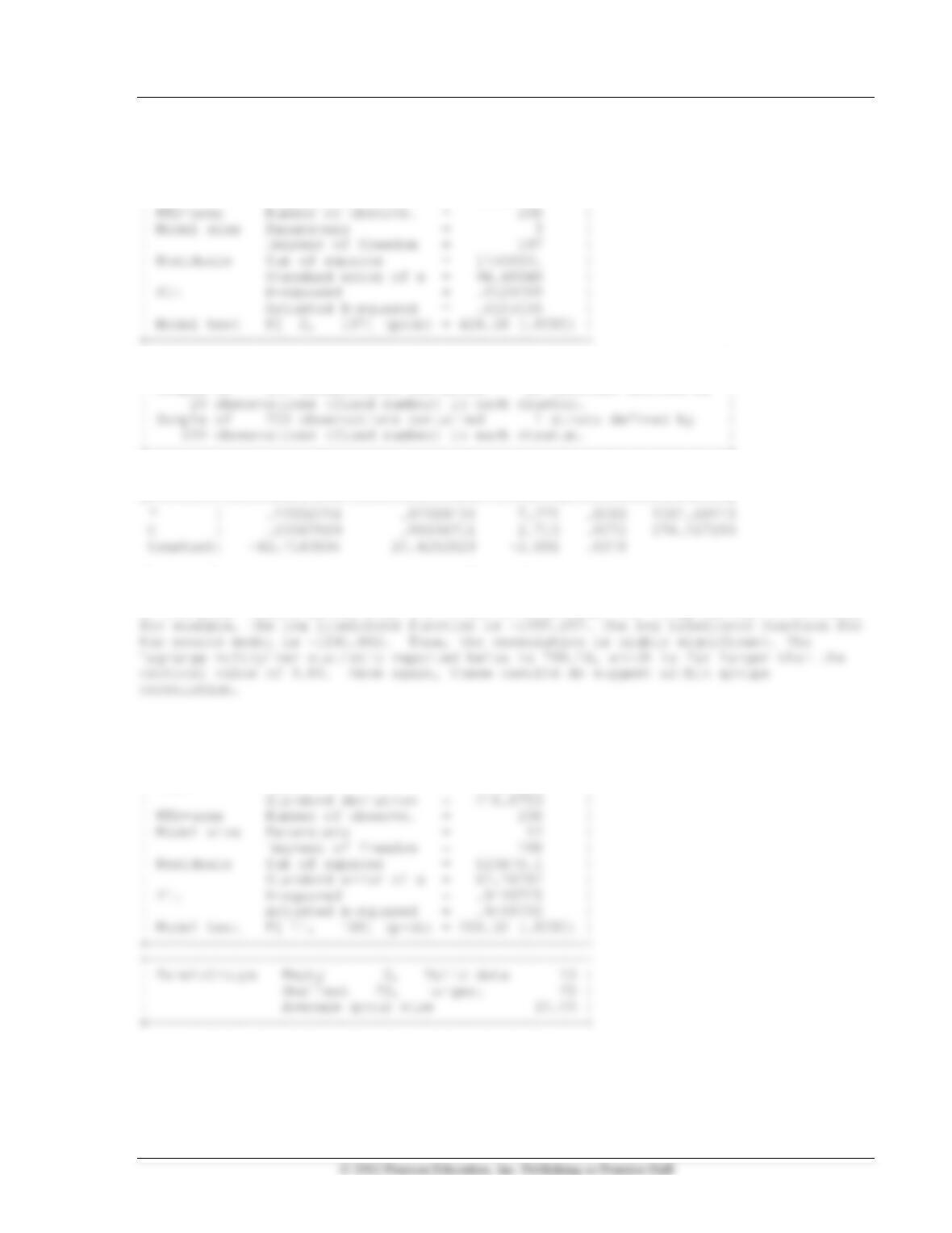
+—————————————————-+
| Ordinary least squares regression |
| LHS=I Mean = 145.9582 |
| Standard deviation = 216.8753 |
| WTS=none Number of observs. = 200 |
| Model size Parameters = 3 |
+——–+————–+—————-+——–+——–+———-+
|Variable| Coefficient | Standard Error |t-ratio |P[|T|>t]| Mean of X|
+——–+————–+—————-+——–+——–+———-+
Chapter 11 Models for Panel Data 103
+—————————————————-+
| Ordinary least squares regression |
| LHS=I Mean = 145.9582 |
| Standard deviation = 216.8753 |
+———————————————————————+
| Covariance matrix for the model is adjusted for data clustering. |
| Sample of 200 observations contained 10 clusters defined by |
+———————————————————————+
+——–+————–+—————-+——–+——–+———-+
|Variable| Coefficient | Standard Error |t-ratio |P[|T|>t]| Mean of X|
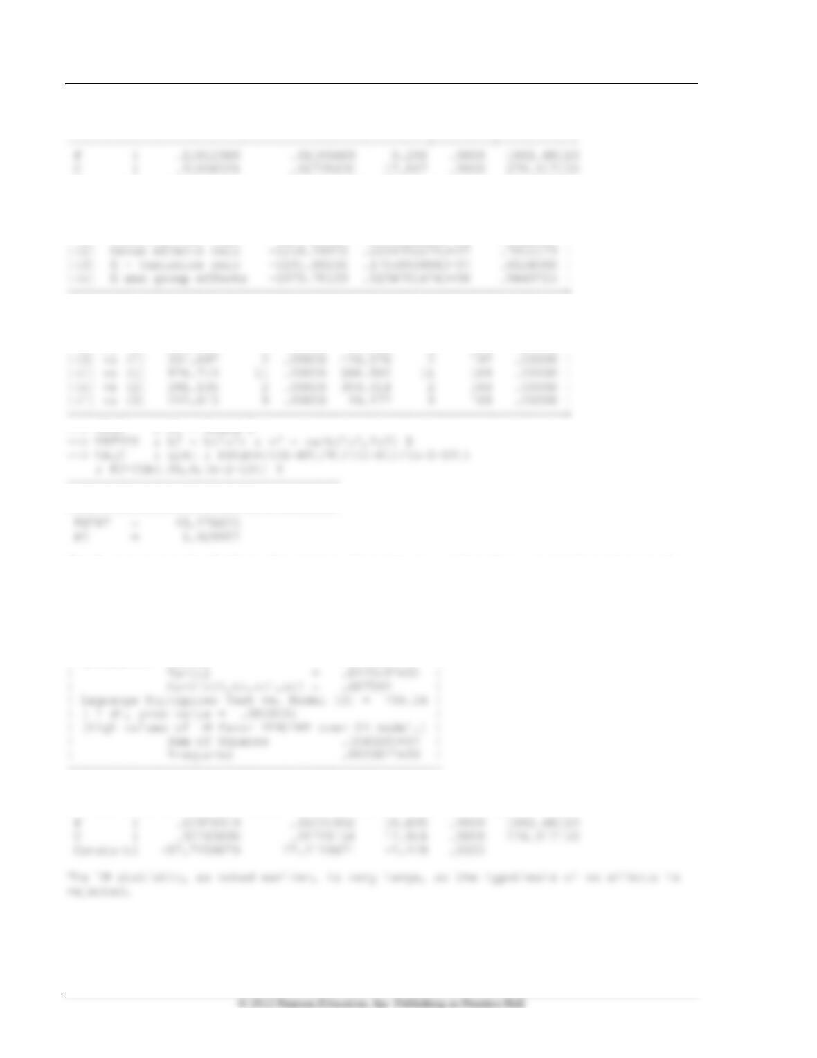
The standard errors increase substantially. This is at least suggestive that there is
correlation across observations within the groups. A formal test would be based on one
of the panel models below. When the random effects model is fit by maximum likelihood,
–> REGRESS ; Lhs = I ; Rhs = F,C,one ; Panel ; Pds=20 ; Fixed $
+—————————————————-+
| Least Squares with Group Dummy Variables |
| Ordinary least squares regression |
| LHS=I Mean = 145.9583 |
104 Greene • Econometric Analysis, Seventh Edition
+——–+————–+—————-+——–+——–+———-+
|Variable| Coefficient | Standard Error |t-ratio |P[|T|>t]| Mean of X|
+——————————————————————–+
| Test Statistics for the Classical Model |
+——————————————————————–+
| Model Log Likelihood Sum of Squares R-squared |
|(1) Constant term only -1359.15096 .9359943929D+07 .0000000 |
+——————————————————————–+
| Hypothesis Tests |
| Likelihood Ratio Test F Tests |
| Chi-squared d.f. Prob. F num. denom. P value |
|(2) vs (1) 285.604 9 .00000 66.932 9 190 .00000 |
+————————————+
| Listed Calculator Results |
The F statistic of 49.18 is far larger than the critical value, so the hypothesis of
equal constant terms is rejected.
–> REGRESS ; Lhs = I ; Rhs = F,C,one
; Panel ; Pds=20 ; Random $
+————————————————–+
| Random Effects Model: v(i,t) = e(i,t) + u(i) |
| Estimates: Var[e] = .278446D+04 |
+————————————————–+
+——–+————–+—————-+——–+——–+———-+
|Variable| Coefficient | Standard Error |b/St.Er.|P[|Z|>z]| Mean of X|
+——–+————–+—————-+——–+——–+———-+
Chapter 11 Models for Panel Data 105
1
+————–
1| 2.45500
–> CALC ; List ; Ctb(.95,2) $
+————————————+
| Listed Calculator Results |
+————————————+
Result = 5.991465
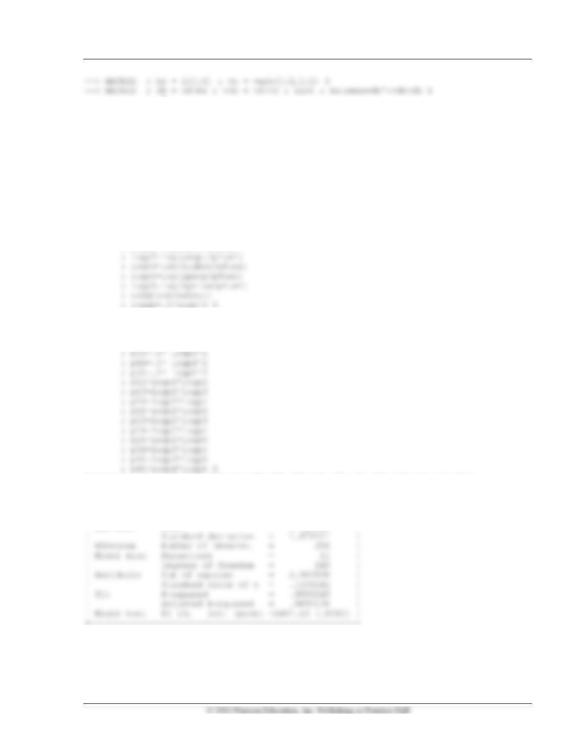
The Hausman statistic is quite small, which suggests that the random effects approach
is consistent with the data.
Application 11.2
create ; logc=log(cost/pfuel)
; logp1=log(pmtl/pfuel)
Namelist ; cd = logp1,logp2,logp3,logp4,logp5 $
create
; p11=.5* logp1^2
; p22=.5* logp2^2
Namelist ; tl = p11,p12,p13,p14,p15,p22,p23,p24,p25,p33,p34,p35,p44,p45,p55$
Namelist ; z = loadfctr,stage,points $
regress;lhs=logc;rhs=one,logq,logq2,cd,z $
+—————————————————-+
| Ordinary least squares regression |
| LHS=LOGC Mean = .7723984 |
+—————————————————-+
106 Greene • Econometric Analysis, Seventh Edition
+——–+————–+—————-+——–+——–+———-+
|Variable| Coefficient | Standard Error |t-ratio |P[|T|>t]| Mean of X|
+——–+————–+—————-+——–+——–+———-+
Constant| 20.3856176 22.8643711 .892 .3735
LOGQ | .95227889 .01832119 51.977 .0000 -1.11237037
LOGQ2 | .06568531 .01060839 6.192 .0000 1.45687077
?
? Turns out the translog model cannot be computed with the firm
? dummy variables. I’ll use the Cobb Douglas form.
?
regress;lhs=logc;rhs= one,logq,logq2,cd ; panel ; pds=ti $
+—————————————————-+
| OLS Without Group Dummy Variables |
| Ordinary least squares regression |
| LHS=LOGC Mean = .7723984 |
| Standard deviation = 1.074424 |
+—————————————————-+
| Panel Data Analysis of LOGC [ONE way] |
| Unconditional ANOVA (No regressors) |
| Source Variation Deg. Free. Mean Square |
+—————————————————-+
+——–+————–+—————-+——–+——–+———-+
|Variable| Coefficient | Standard Error |t-ratio |P[|T|>t]| Mean of X|
+——–+————–+—————-+——–+——–+———-+
LOGQ | .93708702 .01772733 52.861 .0000 -1.11237037
LOGQ2 | .07754607 .01211431 6.401 .0000 1.45687077
+—————————————————-+
| Least Squares with Group Dummy Variables |
| Ordinary least squares regression |
| LHS=LOGC Mean = .7723984 |
| Standard deviation = 1.074424 |
Chapter 11 Models for Panel Data 107
+—————————————————-+
+—————————————————-+
| Panel:Groups Empty 0, Valid data 25 |
| Smallest 2, Largest 15 |
| Average group size 10.24 |
+—————————————————-+
+——–+————–+—————-+——–+——–+———-+
|Variable| Coefficient | Standard Error |t-ratio |P[|T|>t]| Mean of X|
+——–+————–+—————-+——–+——–+———-+
LOGQ | .66448665 .03580894 18.556 .0000 -1.11237037
LOGQ2 | -.00955723 .01280811 -.746 .4563 1.45687077
+——————————————————————–+
| Test Statistics for the Classical Model |
+——————————————————————–+
| Model Log Likelihood Sum of Squares R-squared |
|(1) Constant term only -381.12407 .2943684435D+03 .0000000 |
+——————————————————————–+
| Hypothesis Tests |
| Likelihood Ratio Test F Tests |
| Chi-squared d.f. Prob. F num. denom. P value |
|(2) vs (1) 659.911 24 .00000 117.116 24 231 .00000 |
+——————————————————————–+
+————————————————–+
| Random Effects Model: v(i,t) = e(i,t) + u(i) |
| Estimates: Var[e] = .418468D-02 |
| Var[u] = .127110D-01 |
+————————————————–+
+——–+————–+—————-+——–+——–+———-+
|Variable| Coefficient | Standard Error |b/St.Er.|P[|Z|>z]| Mean of X|
+——–+————–+—————-+——–+——–+———-+
LOGQ | .79769706 .02494671 31.976 .0000 -1.11237037
LOGQ2 | .02011534 .01130089 1.780 .0751 1.45687077
+—————————————————-+
| OLS Without Group Dummy Variables |
| Ordinary least squares regression |
| LHS=LOGC Mean = .7723984 |
| Standard deviation = 1.074424 |
| WTS=none Number of observs. = 256 |
+—————————————————-+
+—————————————————-+
| Panel Data Analysis of LOGC [ONE way] |
| Unconditional ANOVA (No regressors) |
| Source Variation Deg. Free. Mean Square |
| Between 272.013 24. 11.3339 |
+—————————————————-+
+——–+————–+—————-+——–+——–+———-+
|Variable| Coefficient | Standard Error |t-ratio |P[|T|>t]| Mean of X|
+——–+————–+—————-+——–+——–+———-+
LOADFCTR| -.94688632 .18441823 -5.134 .0000 .54786115
STAGE | -.00021794 .402227D-04 -5.418 .0000 507.879666
POINTS | .00199712 .00031682 6.304 .0000 72.9843750
+—————————————————-+
| Least Squares with Group Dummy Variables |
| Ordinary least squares regression |
| LHS=LOGC Mean = .7723984 |
| Standard deviation = 1.074424 |
| WTS=none Number of observs. = 256 |
+—————————————————-+
+—————————————————-+
| Panel:Groups Empty 0, Valid data 25 |
+—————————————————-+
+——–+————–+—————-+——–+——–+———-+
|Variable| Coefficient | Standard Error |t-ratio |P[|T|>t]| Mean of X|
+——–+————–+—————-+——–+——–+———-+
LOADFCTR| -.89457348 .14242570 -6.281 .0000 .54786115
Chapter 11 Models for Panel Data 109
LOGP1 | 1.38217070 .72421015 1.909 .0575 .37999226
+——————————————————————–+
| Test Statistics for the Classical Model |
+——————————————————————–+
| Model Log Likelihood Sum of Squares R-squared |
|(1) Constant term only -381.12407 .2943684435D+03 .0000000 |
+——————————————————————–+
| Hypothesis Tests |
| Likelihood Ratio Test F Tests |
| Chi-squared d.f. Prob. F num. denom. P value |
|(2) vs (1) 659.911 24 .00000 117.116 24 231 .00000 |
|(4) vs (1) 1521.362 34 .00000 2470.054 34 221 .00000 |
|(4) vs (3) 344.355 24 .00000 26.140 24 221 .00000 |
+——————————————————————–+
+————————————————–+
| Random Effects Model: v(i,t) = e(i,t) + u(i) |
| Estimates: Var[e] = .349594D-02 |
| (High values of LM favor FEM/REM over CR model.) |
| Baltagi-Li form of LM Statistic = 170.10 |
+————————————————–+
+——–+————–+—————-+——–+——–+———-+
|Variable| Coefficient | Standard Error |b/St.Er.|P[|Z|>z]| Mean of X|
+——–+————–+—————-+——–+——–+———-+
LOADFCTR| -1.07921018 .13264921 -8.136 .0000 .54786115
STAGE | -.00016415 .672354D-04 -2.441 .0146 507.879666
POINTS | .00044792 .00035950 1.246 .2128 72.9843750