108 Answers to Textbook Questions and Problems
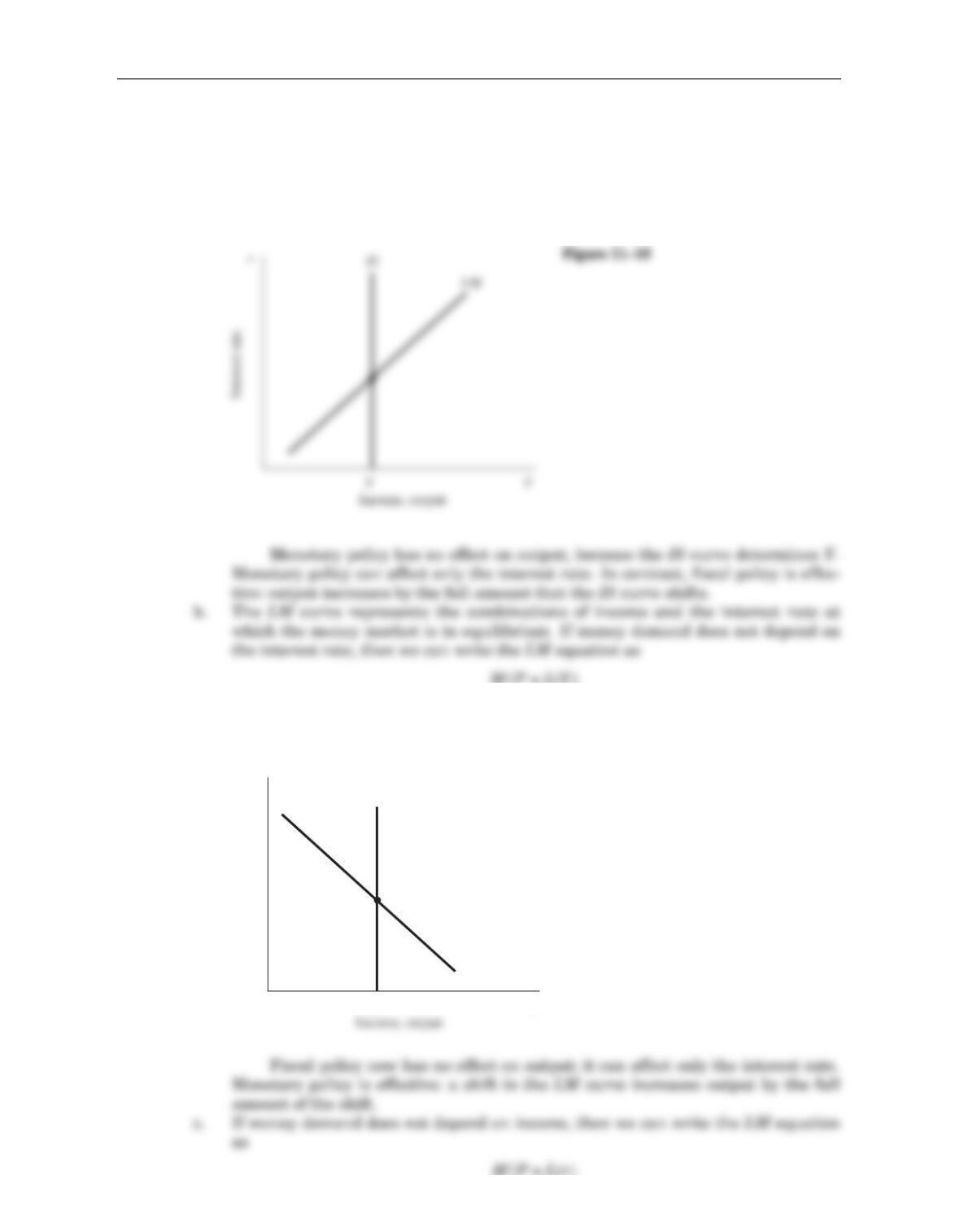
If investment does not depend on the interest rate, then nothing in the IS equa-
tion depends on the interest rate; income must adjust to ensure that the quantity
of goods produced, Y, equals the quantity of goods demanded, C+ I+ G. Thus, the
IS curve is vertical at this level, as shown in Figure 11–16.
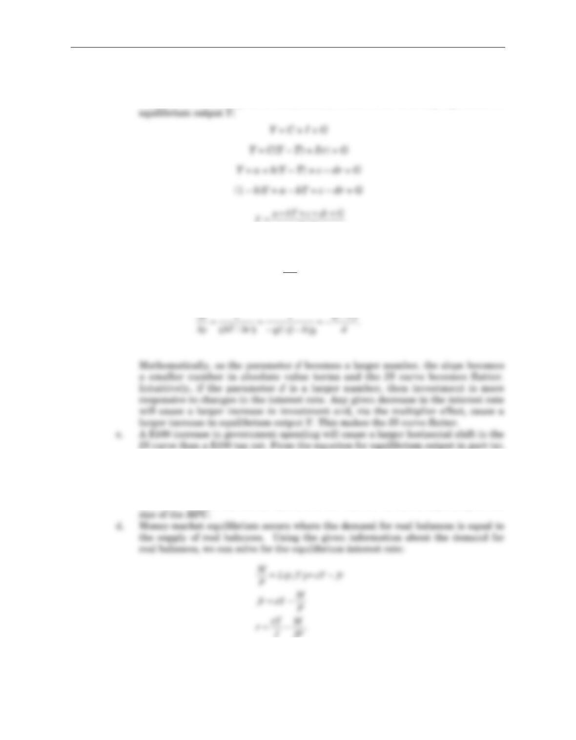
For any given level of real balances M/P, there is only one level of income at
which the money market is in equilibrium. Thus, the LM curve is vertical, as
shown in Figure 11–17.
LM
IS
Y
Y
r
Interest rate
Figure 11–17
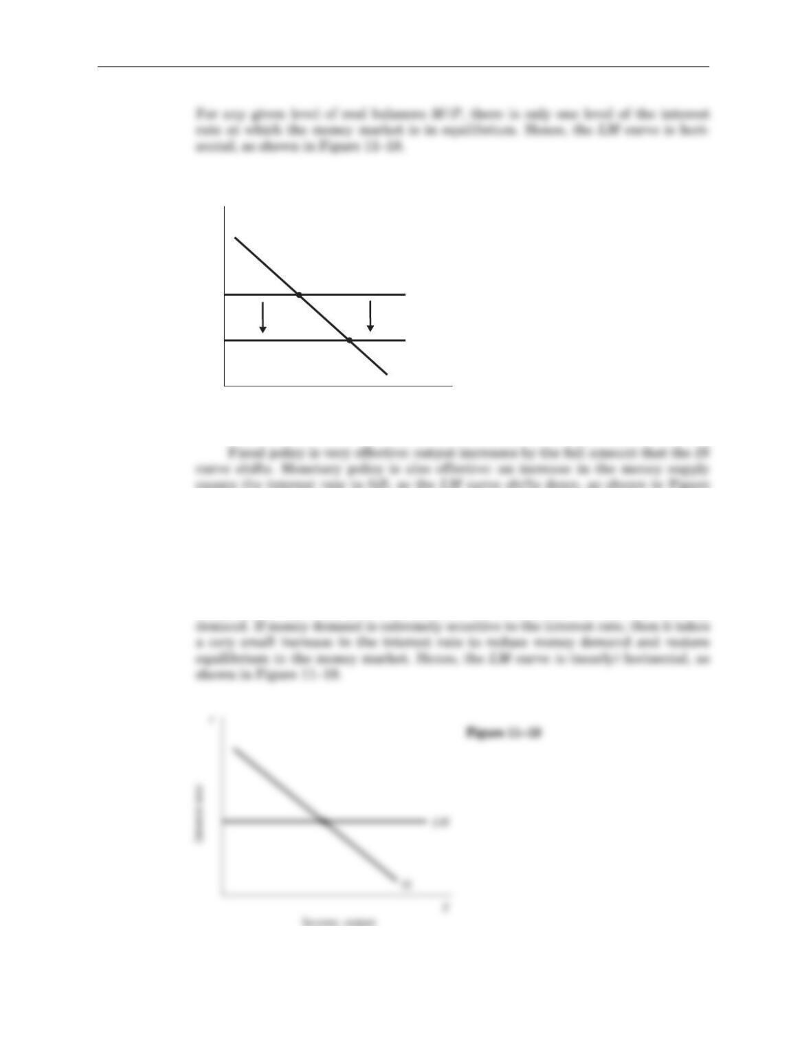
11–18.
d. The LM curve gives the combinations of income and the interest rate at which the
supply and demand for real balances are equal, so that the money market is in
equilibrium. The general form of the LM equation is
M/P = L(r, Y).
Suppose income Yincreases by $1. How much must the interest rate change to
keep the money market in equilibrium? The increase in Yincreases money
Chapter 11 Aggregate Demand II 109
LM1
LM2
IS
Y
Income, output
r
Interest rate
Figure 11–18
An example may make this clearer. Consider a linear version of the LM
equation:
M/P = eY – fr.
Note that as fgets larger, money demand becomes increasingly sensitive to the
interest rate. Rearranging this equation to solve for r, we find
r= (e/f)Y– (1/f)(M/P).
We want to focus on how changes in each of the variables are related to changes in
the other variables. Hence, it is convenient to write this equation in terms of
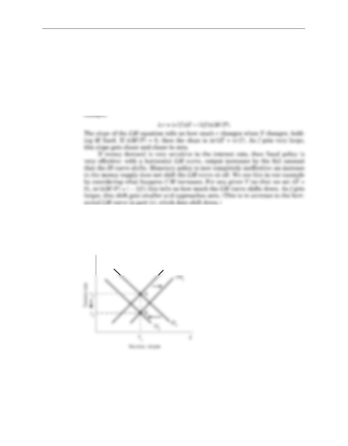
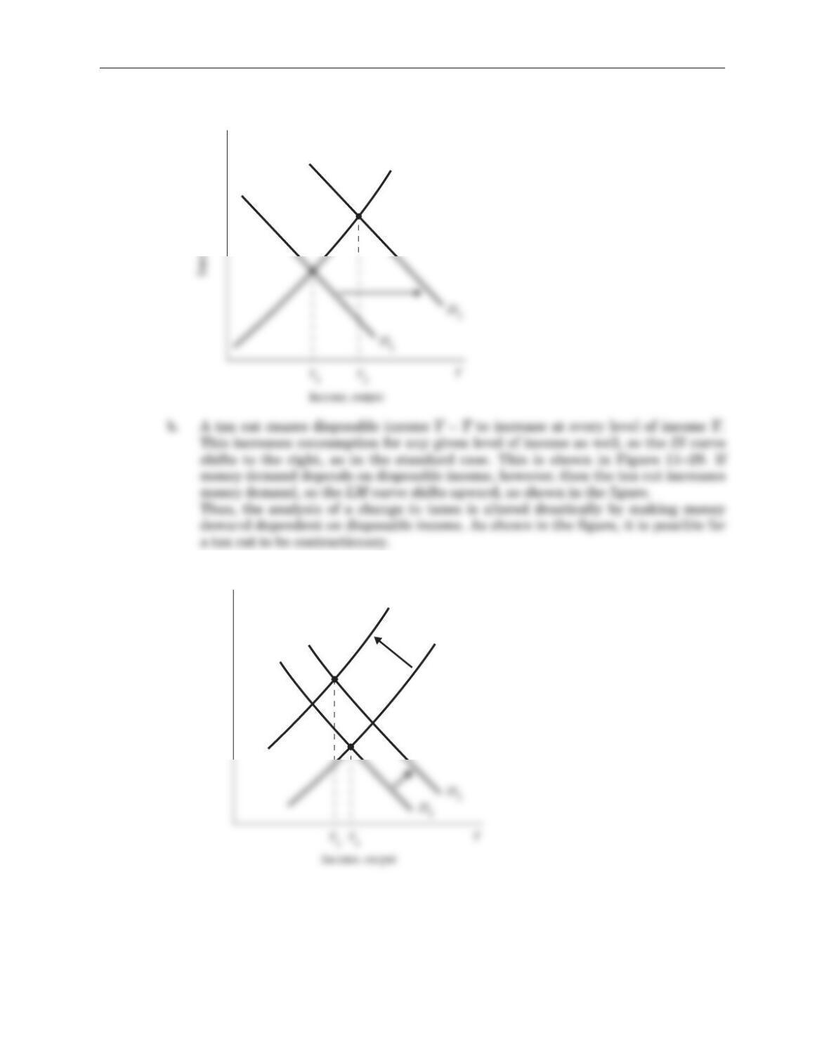
5. To raise investment while keeping output constant, the government should adopt
a loose monetary policy and a tight fiscal policy, as shown in Figure 11–20. In the
new equilibrium at point B, the interest rate is lower, so that investment is high-
er. The tight fiscal policy—reducing government purchases, for example—offsets
the effect of this increase in investment on output.
110 Answers to Textbook Questions and Problems
r
LM1
Figure 11–20
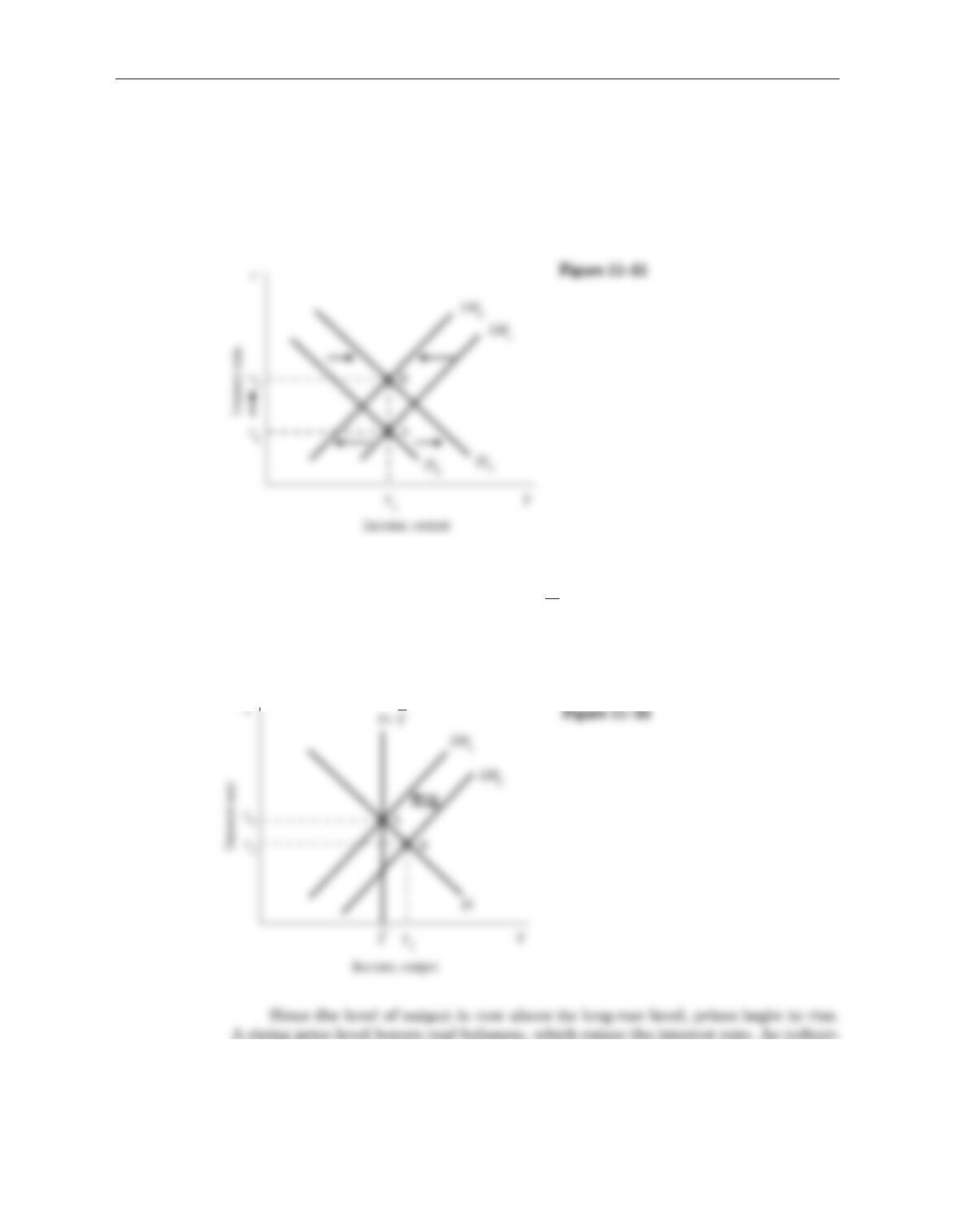
The policy mix in the early 1980s did exactly the opposite. Fiscal policy was
expansionary, while monetary policy was contractionary. Such a policy mix shifts
the IS curve to the right and the LM curve to the left, as in Figure 11–21. The real
interest rate rises and investment falls.
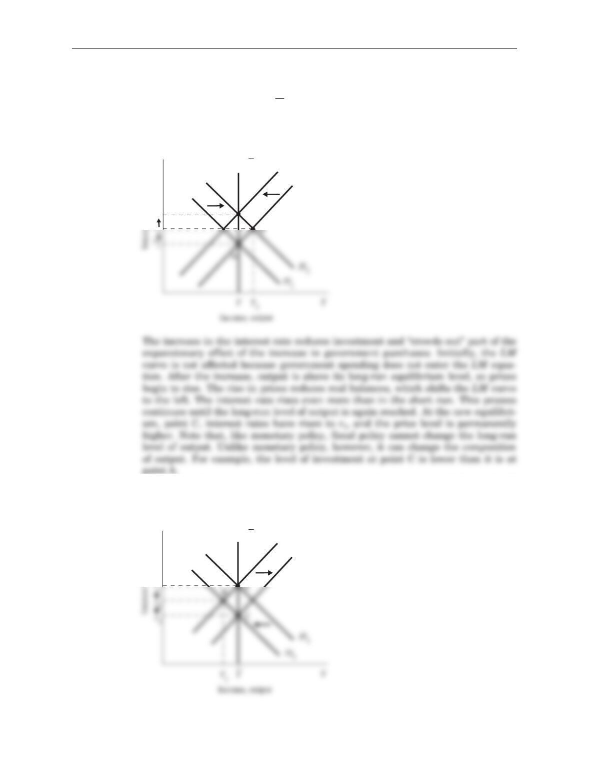
6. a. An increase in the money supply shifts the LM curve to the right in the short run.
This moves the economy from point A to point B in Figure 11–22: the interest rate
falls from r1to r2, and output rises from Yto Y2. The increase in output occurs
because the lower interest rate stimulates investment, which increases output.
ed in Figure 11–22, the LM curve shifts back to the left. Prices continue to rise
until the economy returns to its original position at point A. The interest rate
returns to r1, and investment returns to its original level. Thus, in the long run,
there is no impact on real variables from an increase in the money supply. (This is
what we called monetary neutrality in Chapter 4.)
Chapter 11 Aggregate Demand II 111
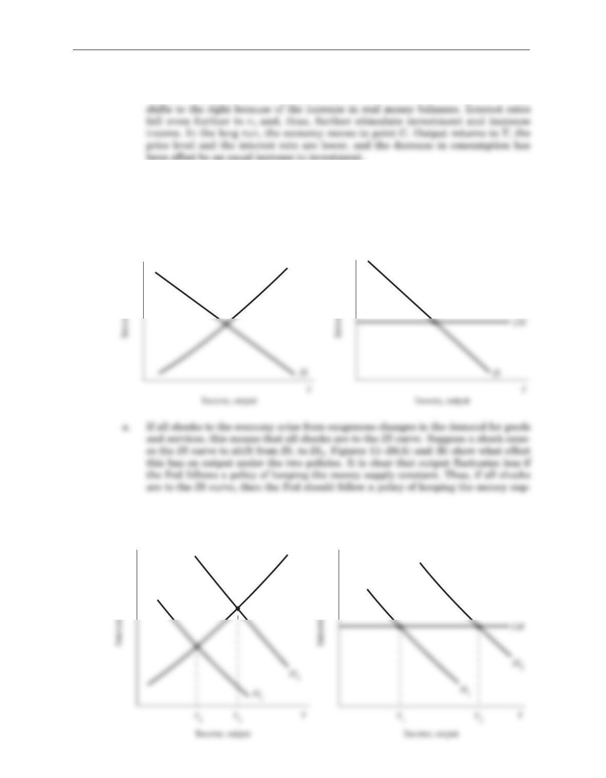
b. An increase in government purchases shifts the IS curve to the right, and the
economy moves from point A to point B, as shown in Figure 11–23. In the short
run, output increases from Yto Y2, and the interest rate increases from r1to r2.
c. An increase in taxes reduces disposable income for consumers, shifting the IS
curve to the left, as shown in Figure 11–24. In the short run, output and the inter-
est rate decline to Y2and r2as the economy moves from point A to point B.
112 Answers to Textbook Questions and Problems
C
r
r3
r2
LM2
LM1
Y= Y
Figure 11–23
r
Y= Y
LM2
LM1
Figure 11–24
Initially, the LM curve is not affected. In the longer run, prices begin to decline
because output is below its long-run equilibrium level, and the LM curve then
7. Figure 11–25(A) shows what the IS–LM model looks like for the case in which the Fed
holds the money supply constant. Figure 11–25(B) shows what the model looks like if
the Fed adjusts the money supply to hold the interest rate constant; this policy makes
the effective LM curve horizontal.
Chapter 11 Aggregate Demand II 113
LM
A. Holding the Money Supply Constant B. Holding the Interest Rate Constant
r
r
Figure 11–25
r
LM
r
A. Holding the Money Supply Constant B. Holding the Interest Rate Constant
Figure 11–26
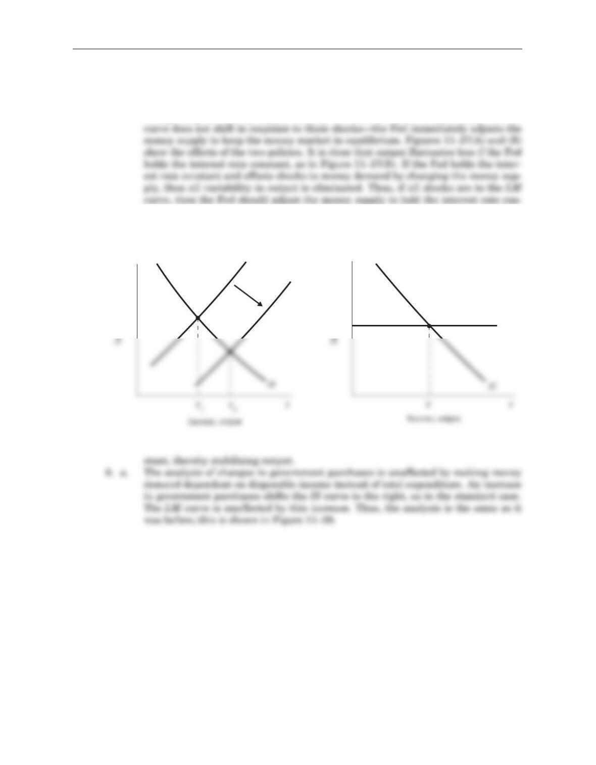
114 Answers to Textbook Questions and Problems
ply constant.
b. If all shocks in the economy arise from exogenous changes in the demand for
money, this means that all shocks are to the LM curve. If the Fed follows a policy
of adjusting the money supply to keep the interest rate constant, then the LM
A. Holding the Money Supply Constant
r
B. Holding the Interest Rate Constant
r
LM
LM1
LM2
Figure 11–27
Chapter 11 Aggregate Demand II 115
B
A
r
Interest rate
LM1
LM2
Figure 11–29
LM
r
Figure 11–28
9. a. The goods market is in equilibrium when output is equal to planned expenditure,
or Y= PE. Starting with this equilibrium condition, and making the substitutions
from the information given in the problem, results in the following expression for
b. The slope of the IS curve is measured as
From the equation in part (a), the slope of the IS curve can be found as follows:
note that the impact of the tax cut depends on the marginal propensity to con-
sume, as given by the parameter b. If the MPC is 0.75, for example, then a $100
tax cut will shift the IS curve by only $75. Intuitively, this makes sense because
the entire $100 increase in government spending will be spent, whereas only a
portion of the tax cut will be spent, and the rest will be saved depending on the
116 Answers to Textbook Questions and Problems
b
–1
D
D
r
Y.
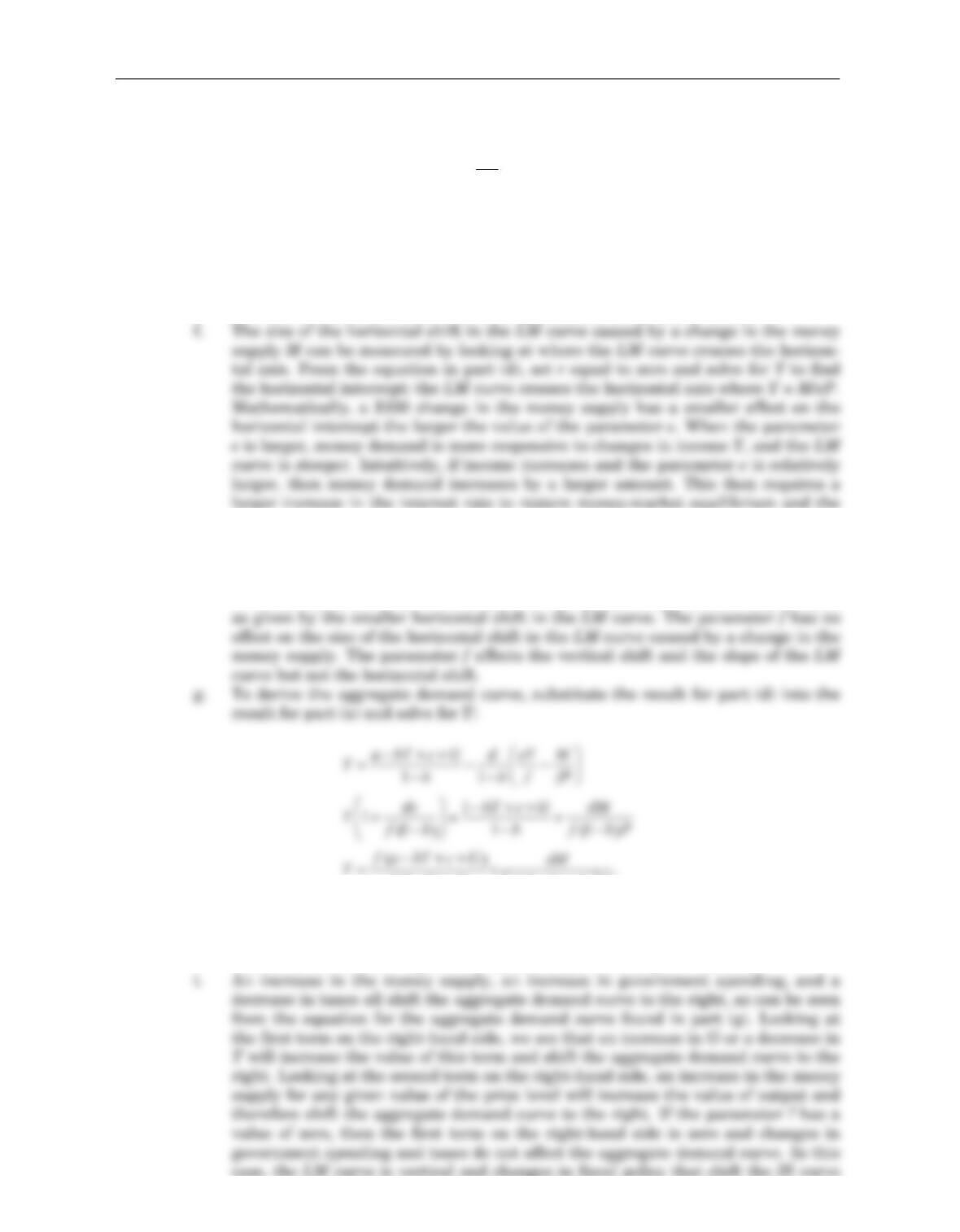
e. The slope of the LM curve is measured as
From the equation in part (d), the slope of the LM curve is e/f. As the parameter f
becomes a larger number, the slope becomes smaller and the LM curve becomes
flatter. Intuitively, as the parameter fbecomes a larger number, money demand is
more responsive to changes in the interest rate. This means that any increase in
income that leads to an increase in money demand will require a relatively small
increase in the interest rate to restore equilibrium in the money market.
LM curve becomes relatively steeper. Overall, the increase in the money supply
will lower the interest rate and increase investment spending and output. When
output rises, so does money demand, and if the parameter eis relatively large,
then the interest rate will need to rise by a larger amount to restore equilibrium
in the money market. The overall effect on equilibrium output is relatively smaller,
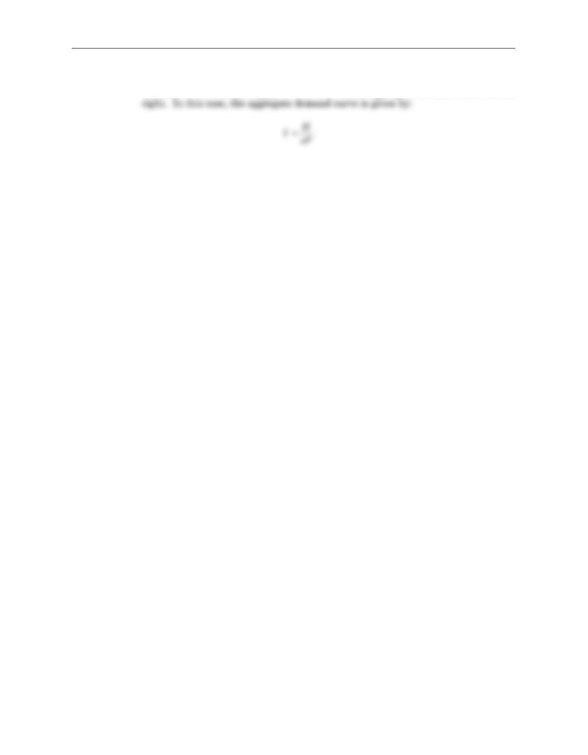
h. The aggregate demand curve has a negative slope, as can be seen from the equa-
tion in part (g) above. An increase in the price level Pwill decrease the value of
the second term on the right-hand side, and therefore output Ywill fall.
Chapter 11 Aggregate Demand II 117
D
D
r
Y.
–
()
++–
()
+
È
΢
˚
fbde
f b de P
11.
have no effect on output. Monetary policy is still effective in this case, and an
increase in the money supply will still shift the aggregate demand curve to the
118 Answers to Textbook Questions and Problems