A n s w e r s t o t h e R e v i e w Q u i z z e s
Page 269 (page 677 in Economics)
1. Which components of aggregate expenditure are influenced by real GDP?
2. Define and explain how we calculate the marginal propensity to consume and the marginal
propensity to save.
3. How do we calculate the effects of real GDP on consumption expenditure and imports by using
the marginal propensity to consume and the marginal propensity to import?
The effects of real GDP on consumption expenditure and imports are determined respectively by the
Page 273 (page 681 in Economics)
1. What is the relationship between aggregate planned expenditure and real GDP at equilibrium
expenditure?
2. How does equilibrium expenditure come about? What adjusts to achieve equilibrium?
Equilibrium expenditure results from adjustments in real GDP. For instance, if aggregate planned
3. If real GDP and aggregate expenditure are less than equilibrium expenditure, what happens to
firms’ inventories? How do firms change their production? And what happens to real GDP?
11
EXPENDITURE
MULTIPLIERS**
C h a p t e r
4. If real GDP and aggregate expenditure are greater than equilibrium expenditure, what happens to
firms’ inventories? How do firms change their production? And what happens to real GDP?
Page 278 (page 686 in Economics)
1. What is the multiplier? What does it determine? Why does it matter?
2. How do the marginal propensity to consume, the marginal propensity to import, and the income
tax rate influence the multiplier?
3. How do fluctuations in autonomous expenditure influence real GDP?
Page 283 (page 691 in Economics)
1. How does a change in the price level influence the AE curve and the AD curve?
2. If autonomous expenditure increases with no change in the price level, what happens to the AE
curve and the AD curve? Which curve shifts by an amount that is determined by the multiplier and
why?
3. How does an increase in autonomous expenditure change real GDP in the short run? Does real
GDP change by the same amount as the change in aggregate demand? Why or why not?
4. How does real GDP change in the long run when autonomous expenditure increases? Does real
GDP change by the same amount as the change in aggregate demand? Why or why not?
E X P E N D I T U R E M U L T I P L I E R S 1 4 1
Page 289 (page 697 in Economics)
In an economy, autonomous consumption expenditure is $50 billion, investment is $200 billion, and
government expenditure is $250 billion. The marginal propensity to consume is 0.7 and net taxes are
$250 billion. Exports are $500 billion and imports are $450 billion. Assume that net taxes and imports
are autonomous and the price level is fixed.
a. What is the consumption function?
b. What is the equation of the AE curve?
The equation of the AE curve is AE = 375 + 0.7Y, where Y is real GDP and the 375 is $375 billion.
Aggregate planned expenditure is the sum of consumption expenditure, investment, government
c. Calculate equilibrium expenditure.
Equilibrium expenditure is $1,250 billion. Equilibrium expenditure is the level of aggregate expenditure
e. If investment decreases to $150 billion, what is the change in equilibrium expenditure?
f. Describe the process in part (e) that moves the economy to its new equilibrium expenditure.
When investment decreases by $50 billion, aggregate planned expenditure is less than real GDP. Firms
1 4 2 C H A P T E R 1 1
A n s w e rs t o t he S t u dy P l an P ro b l e m s a n d A pp li c at io n s
1. In an economy, when income increases from $400 billion to $500 billion, consumption
expenditure changes from $420 billion to $500 billion. Calculate the marginal propensity to
consume, the change in saving, and the marginal propensity to save.
The marginal propensity to consume is the fraction of a change in disposable income that is consumed.
In this economy, when income increases by $100 billion per year, consumption expenditure increases
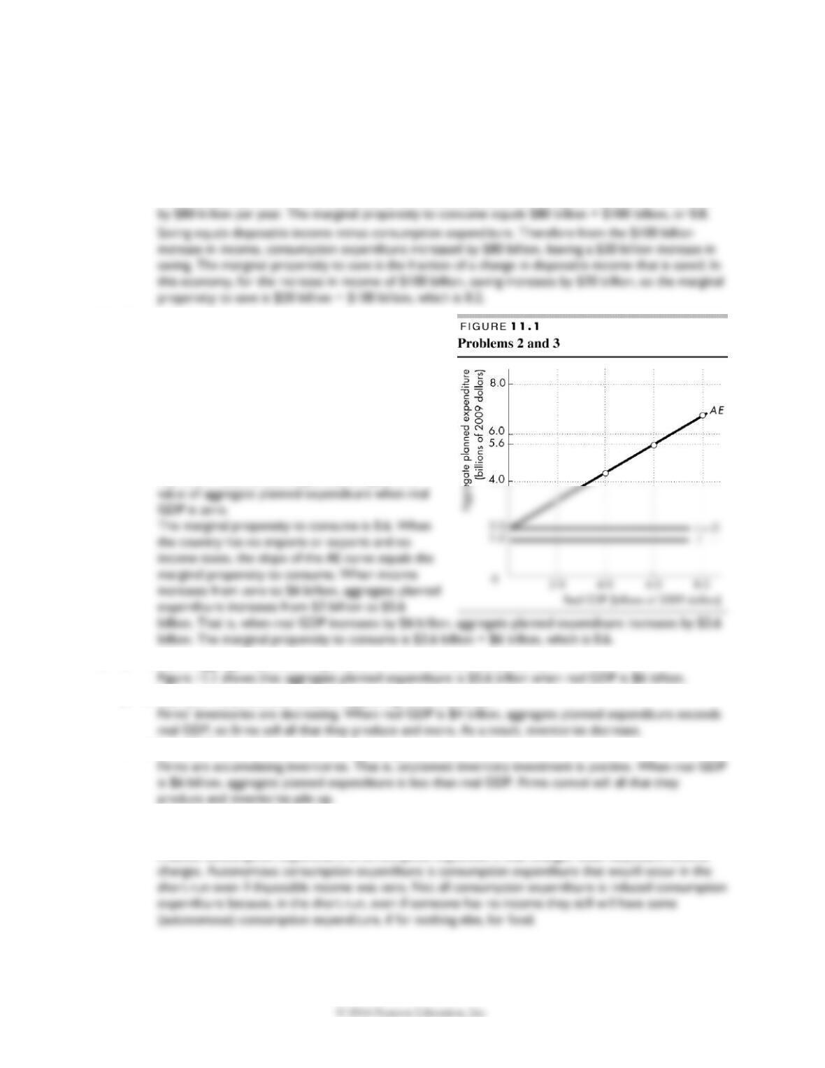
Use Figure 11.1 to work Problems 2 and 3.
Figure 11.1 illustrates the components of aggregate
planned expenditure on Turtle Island. Turtle Island has
no imports or exports, no incomes taxes, and the price
level is fixed.
2. Calculate autonomous expenditure and the
marginal propensity to consume.
Autonomous expenditure is $2 billion. Autonomous
expenditure is expenditure that does not depend on
real GDP. Autonomous expenditure equals the
3. a. What is aggregate planned expenditure when real GDP is $6 billion?
b. If real GDP is $4 billion, what is happening to inventories?
c. If real GDP is $6 billion, what is happening to inventories?
4. Explain the difference between induced consumption expenditure and autonomous consumption
expenditure. Why isn’t all consumption expenditure induced expenditure?
Induced consumption expenditure is consumption expenditure that changes when disposable income
5. Explain how an increase in business investment at a constant price level changes equilibrium
expenditure.
Use the following data to work Problems 6 and 7.
An economy has a fixed price level, no imports, and no income taxes. MPC is 0.80, and real GDP is $150
billion. Businesses increase investment by $5 billion.
6. Calculate the multiplier and the change in real GDP.
With no imports and no income taxes, the multiplier equals 1/(1 MPC). So the multiplier is 1/(1
7. Calculate the new real GDP and explain why real GDP increases by more than $5 billion.
Real GDP was initially $150 billion. The increase in investment increased real GDP by $25 billion, so
8. An economy has a fixed price level, no imports, and no income taxes. An increase in autonomous
expenditure of $2 trillion increases equilibrium expenditure by $8 trillion. Calculate the multiplier
and explain what happens to the multiplier if an income tax is introduced.
The multiplier is defined as the change in equilibrium expenditure divided by the change in autonomous
Use the following data to work Problems 9 to 13.
Suppose that the economy is at full employment, the price level is 100, and the multiplier is 2.
Investment increases by $100 billion.
9. What is the change in equilibrium expenditure if the price level remains at 100?
10. a. What is the immediate change in the quantity of real GDP demanded?
b. In the short run, does real GDP increase by more than, less than, or the same amount as the
immediate change in the quantity of real GDP demanded?
11. In the short run, does the price level remain at 100? Explain why or why not.
12. a. In the long run, does real GDP increase by more than, less than, or the same amount as the
immediate increase in the quantity of real GDP demanded?
1 4 4 C H A P T E R 1 1
b. Explain how the price level changes in the long run.
13. Are the values of the multipliers in the short run and the long run larger or smaller than 2?
14. Use the data in the Worked Problem on p. 287 (page 699 in Economics). Calculate the change in
equilibrium expenditure when investment decreases by $150 billion.
E X P E N D I T U R E M U L T I P L I E R S 1 4 5
100
25
200
50
300
75
400
100
200
300
225
Answers to Additional Problems and Applications
Use the following data to work Problems 15 and 16.
You are given the information in the table about the economy of
Australia.
15. Calculate the marginal propensity to save.
The marginal propensity to save is the fraction of a change in
16. Calculate consumption at each level of disposable income. Calculate the marginal propensity to
consume.
The table to the right shows Australia’s consumption
Use the following news clip to work Problems 17 to 19.
Americans $2.4 trillion Poorer
The Federal Reserve reported that household wealth decreased by $2.4 trillion or $21,000 per
household in the third quarter of 2011. This drop is the steepest since 2008 and the second consecutive
quarterly drop. Foreclosures lowered household debt slightly but credit card debt increased. Many
households are struggling to buy the essentials and spending on food has decreased. Separately, the
Bureau of Economic Analysis reported that consumption expenditure increased by $39 billion in the
third quarter of 2011.
Sources: The New American, December 11, 2011 and the Bureau of Economic Analysis
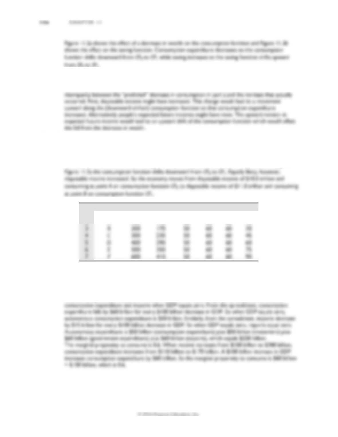
17. Explain and draw a graph to illustrate how a fall in household wealth would be expected to influence the
consumption function and saving function.
Disposable
income
Saving
(billions of dollars per year)
0
0
400
300
18. What factors might explain the actual changes in consumption expenditure and wealth that
occurred in the third quarter of 2011?
According to the article, consumption increased. At least two other factors could explain the
19. Draw a graph of a consumption function and show at what points consumers were actually
operating in the second and third quarters. Make any necessary assumptions and explain your
answer.
Regardless of any increase in future expected income, it is likely the case that the decrease in wealth led
to a net downward shift of the consumption function because the decrease in wealth was so large. In
A
B
C
D
E
F
G
1
Y
C
I
G
X
M
2
A
100
110
50
60
60
15
3
B
200
170
50
60
60
30
4
5
400
290
50
60
60
60
6
E
500
350
50
60
60
75
7
600
410
50
60
60
90
Use the spreadsheet above, which lists real GDP (Y ) and the components of aggregate planned
expenditure in billions of dollars, to work Problems 20 and 21.
20. Calculate autonomous expenditure. Calculate the marginal propensity to consume.
Autonomous expenditure equals the value of aggregate planned expenditure when real GDP is zero.
Because the spreadsheet does not list GDP of zero, we must extrapolate to calculate the value of
21. a. What is aggregate planned expenditure when real GDP is $200 billion?
Aggregate planned expenditure is $310 billion. Aggregate planned expenditure is the sum of
b. If real GDP is $200 billion, explain the process that moves the economy toward equilibrium
expenditure.
Inventories are decreasing so that the unplanned inventory change is negative. When real GDP is $200
c. If real GDP is $500 billion, explain the process that moves the economy toward equilibrium
expenditure.
22. Wholesale Inventories Decline, Sales Rise
The Commerce Department reported that wholesale inventories fell 1.3 percent in August for a
record 12th consecutive month, evidence that companies are trimming orders to factories, which
helped depress economic output during the recession. Economists hope that the rising sales will
encourage businesses to begin restocking their inventories, which would boost factory production
and help bolster broad economic growth in coming months.
Source: The New York Times, October 8, 2009
Explain why a fall in inventories is associated with recession and a restocking of inventories might
bolster economic growth.
23. Obama’s New Stimulus
The Obama recovery plan announced on Monday includes proposed spending of $50 billion to
rebuild 150,000 miles of roads, construct and maintain 4,000 miles of rail, and fix or rebuild 150
miles of runways.
Source: USA Today, September 10, 2010
If the slope of the AE curve is 0.7, calculate the immediate change in aggregate planned
expenditure and the change in real GDP in the short run if the price level remains unchanged.
24. Obama’s Economic Recovery Plan
President Obama’s proposal to jolt a listless recovery with $180 billion worth of tax breaks and
transportation projects left economists largely unimpressed Tuesday.
Source: USA Today, September 10, 2010
If taxes fall by $90 billion and the spending on transport projects increases by $90 billion, which
component of Obama’s recovery plan would have the larger effect on equilibrium expenditure,
other things remaining the same?
The spending on transportation projects will have the larger effect because the expenditure multiplier is
Use the following news item to work Problems 25 to 27.
The BEA reported that in the third quarter of 2014 U.S.
exports increased by $40 billion.
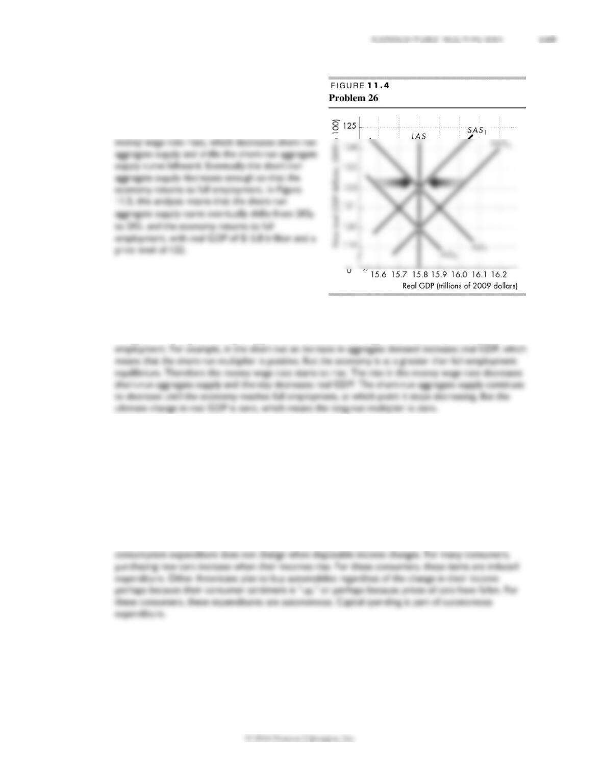
25. Explain and draw a graph to illustrate the effect of
an increase in exports on equilibrium expenditure
in the short run.
The increase in exports increases aggregate
expenditure because exports is a component of
6. Explain and draw a graph to illustrate the effect of an
increase in exports on equilibrium real GDP in the short
run.
The increase in exports increases aggregate
27. Explain and draw a graph to illustrate the effect of
an increase in exports on equilibrium real GDP in
the long run.
In the short run, the economy is in an above full-
employment equilibrium. As time passes, the
28. Compare the multiplier in the short run and the long run and explain why they are not identical.
The long-run multiplier is zero, which means that the short-run multiplier is larger than the long-run
multiplier. The long-run multiplier equals zero because in the long run the economy returns to full
Use the following news clip to work Problems 29 to 31.
Consumer Sentiment in U.S. Rose to Three Month High
Consumer sentiment was up in August helped by merchant discounts, especially from auto dealerships
who received incentives from automakers Honda, General Motors, and Toyota to lower prices.
But consumers are worried about the future. They are worried about tax changes and government
budget cuts that are on the horizon. Capital spending fell somewhat.
Source: Bloomberg, September 1, 2012
29. Which of the expenditures listed in the news clip are part of induced expenditure and which is
part of autonomous expenditure?
Induced consumption expenditure changes with changes in disposable income. Autonomous
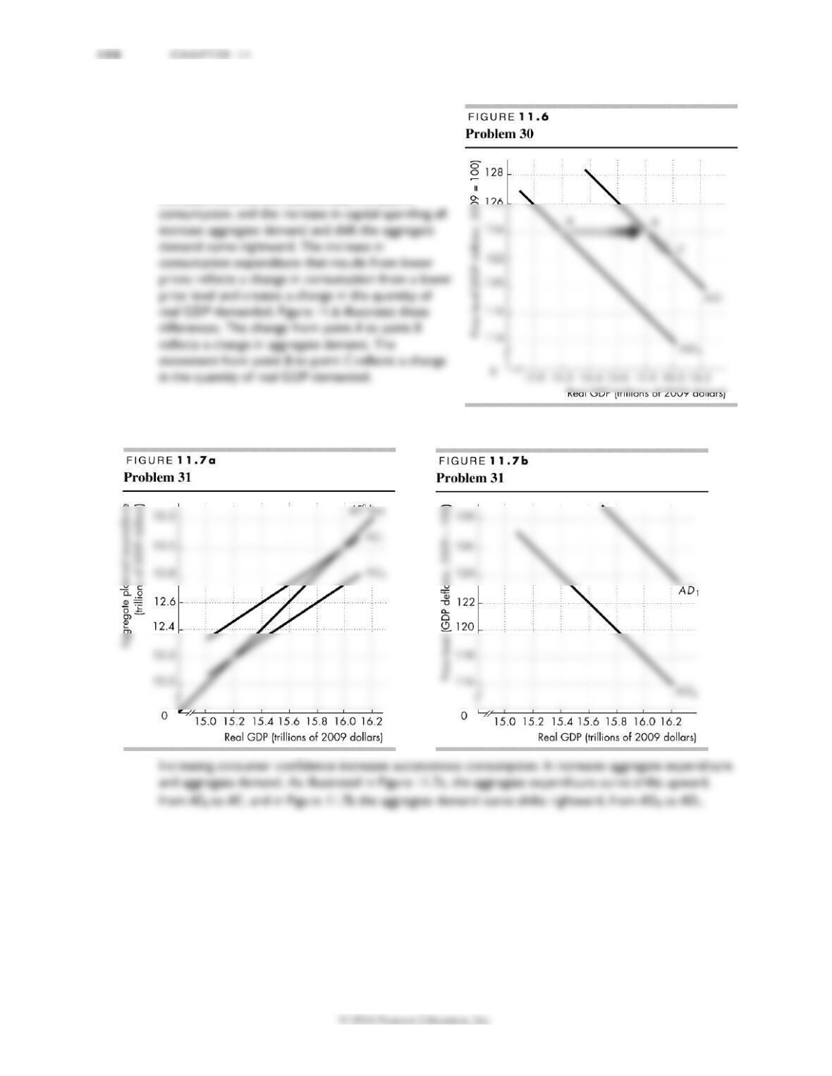
30. Which of the events reported in the news clip
would change aggregate demand and which would
change the quantity of real GDP demanded?
Provide a graphical illustration of the distinction.
The increase in consumption expenditure induced by
increased income, the autonomous increase in
31. Explain and draw a graph to illustrate how
increasing consumer confidence influences aggregate expenditure and aggregate demand.
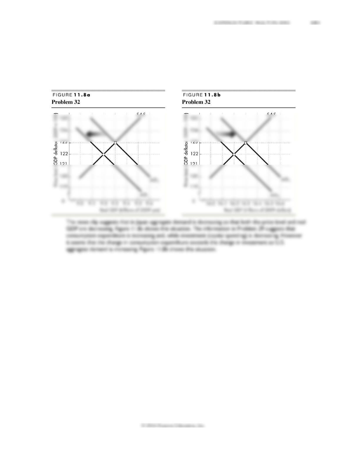
32. Japan Slides Into Recession
In Japan, consumer prices slid at a faster pace in July and industrial production unexpectedly
slumped.
Source: Bloomberg, September 1, 2012
Contrast what the news clip says is happening in Japan with what is happening in the United States
in Problem 29 and provide a graphical analysis of the differences.
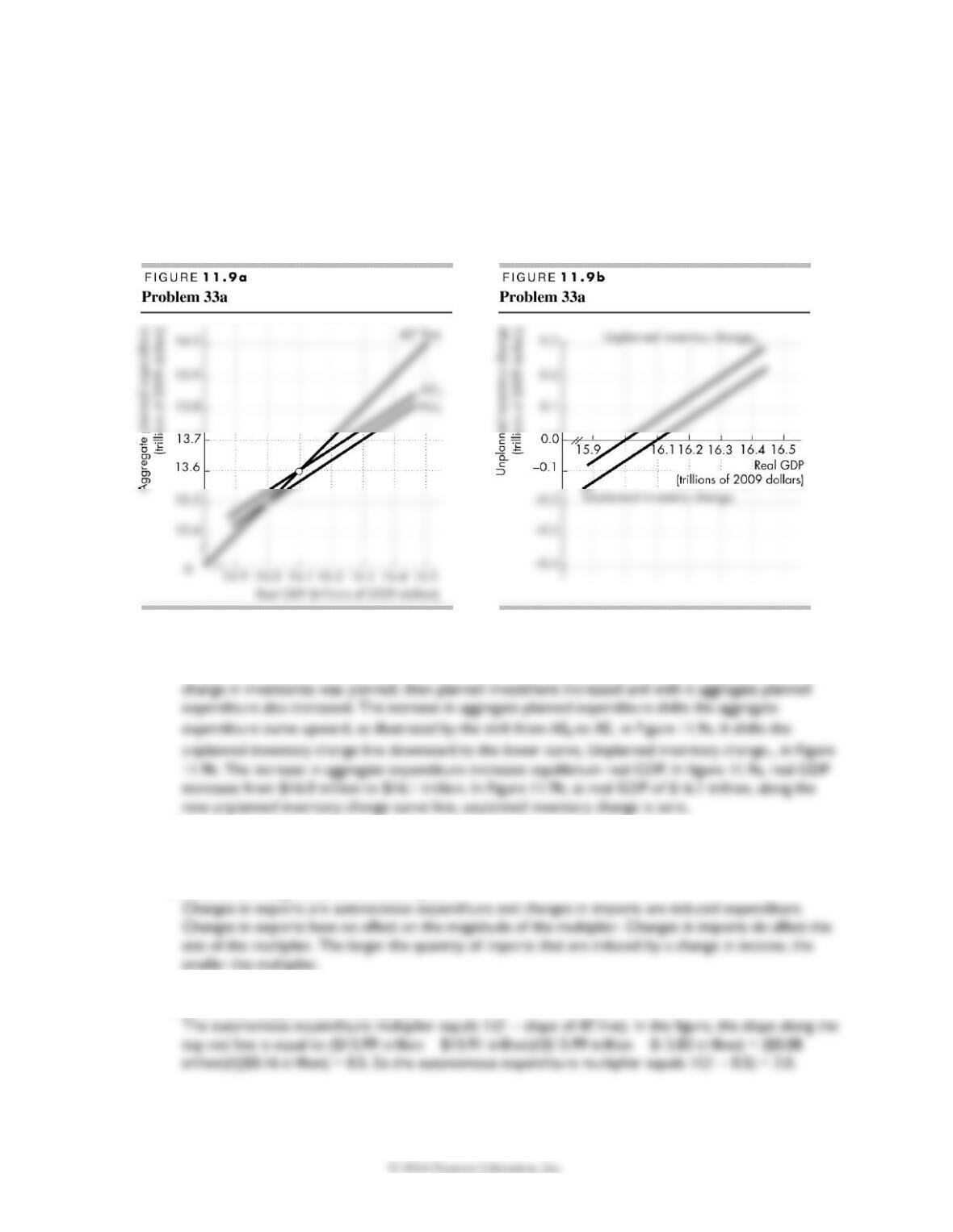
1 5 2 C H A P T E R 1 1
Economics in the News
33. After you have studied Economics in the News on pp. 284–285 (692–693 in Economics), answer the
following questions.
a. If the 2014 changes in inventories were mainly planned changes, what role did they play in
shifting the AE curve and changing equilibrium expenditure? Use a two-part figure (similar to that
on p. 272 (p. 680 in Economics)) to answer this question.
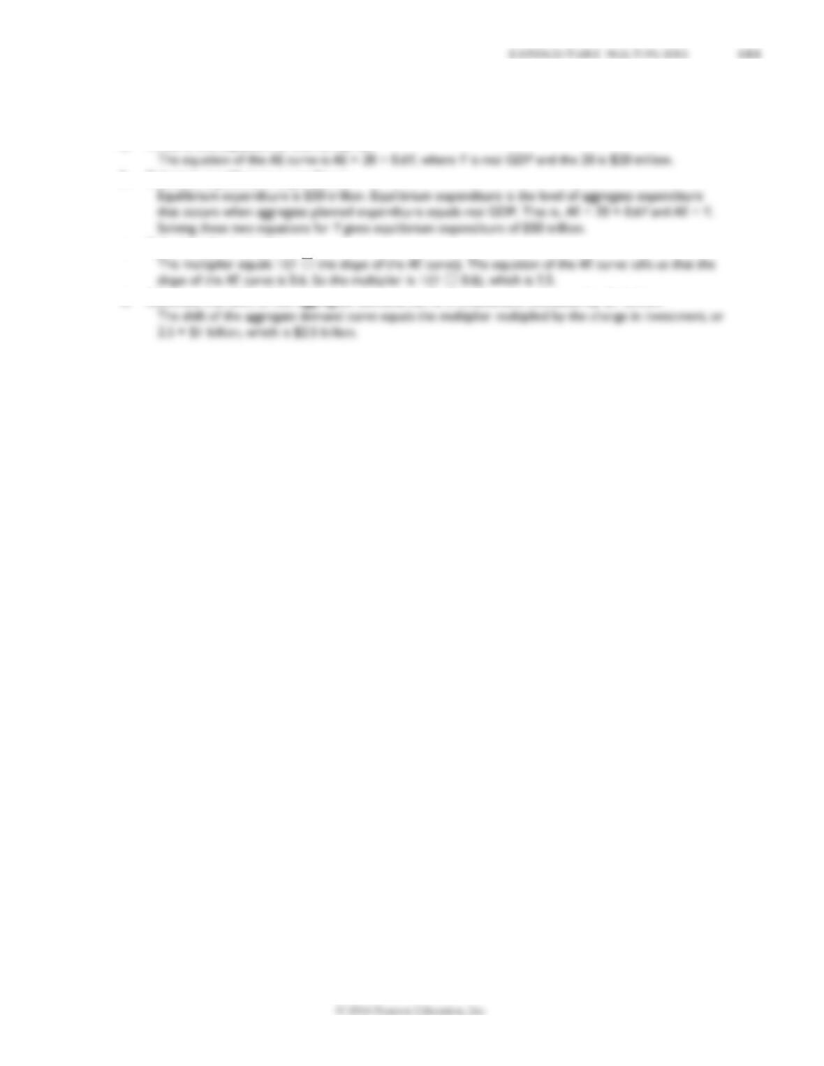
Figure 11.9a shows aggregate planned expenditure; Figure 11.9b shows unplanned inventory change.
When aggregate planned expenditure is given by AE0, unplanned inventory change is equal to zero when
real GDP is $16.0 trillion, so unplanned inventory change is given by the top line in Figure 11.9b. If the
b. The BEA news release reports that exports of goods and services were up 10.1 percent and
imports of goods and services were up 11.0 percent. Were these increases in expenditure
increases in autonomous expenditure or increases in induced expenditure, and how do they
influence the magnitude of the multiplier?
c. Using the assumptions made in Figure 2 on p. 285 (p. 693 in Economics), what is the value of the
autonomous expenditure multiplier?
34. In an economy with a fixed price level, autonomous spending is $20 trillion and the slope of the
AE curve is 0.6.
a. What is the equation of the AE curve?
b. Calculate equilibrium expenditure.
c. Calculate the multiplier.
d. Calculate the shift of the aggregate demand curve if investment increases by $1 billion.