22 Topics in International Macroeconomics
Notes to Instructor
Chapter Summary
This chapter covers extensions to the models presented in earlier chapters. There are four
topics covered:
■ purchasing power parity (PPP), especially the issue of why price levels are higher
in richer countries;
■ uncovered interest parity (UIP), and the implications of the fact that forex traders
seem to make positive net profits;
■ The problem of government defaults, including issues of supply and demand for
loans to governments and the cost of default to the defaulting government; and
■ the performance of the global macroeconomy before, during, and after the 2007–
2009 global financial crisis and the Great Recession.
Comments
This chapter provides extensions to earlier models presented in the textbook. These
sections can be presented independently. There are some connections made between the
sections in the conclusion following each, and in the conclusion section for the chapter.
The sections build on the theories and empirical analysis from earlier in the textbook. An
alternative approach to these sections would be to cover each section immediately after
the chapters on which they expand.
1. Exchange Rates in the Long Run: Deviations from Purchasing Power Parity.
This section presents an extension of the relative PPP model. It describes the
2. Exchange Rates in the Short Run: Deviations from Uncovered Interest
Parity. This section reconsiders empirical tests of the UIP condition and the
reasons arbitrage may fail in financial markets (trade costs, risk‒return trade–offs,
3. Debt and Default. This section models the repayment of sovereign debt as a
contingent claim based on the benefits and costs of default. The costs of default
4. Case Study: The Global Macroeconomy and the Global Financial Crisis. This
section begins with a review of the behavior of emerging market (EM) economies
since 1997. These economies dramatically increased their stock of foreign
exchange reserves as insurance against currency crises. To do this, they ran
current account surpluses. Thus, EM countries were the lenders. Developed
market (DM) economies were the borrowers. Much of this massive flow was used
to purchase U.S. Treasury securities. Yields on those securities fell, investors
An outline of the chapter follows.
1. Exchange Rates in the Long Run: Deviations from Purchasing Power Parity
a. Limits to Arbitrage
i. Trade Costs in Practice
b. Application: It’s Not Just the Burgers That Are Cheap
c Nontraded Goods and the Balassa‒Samuelson Model
i. A Simple Model
d. Overvaluations, Undervaluations, and Productivity Growth: Forecasting
Implications for Real and Nominal Exchange Rates
i. Forecasting the Real Exchange Rate
ii. Convergence
iii. Trend
iv. Convergence + Trend
v. Forecasting the Nominal Exchange Rate
vi. Adjustment to Equilibrium
e. Application: Real Exchange Rates in Emerging Markets
i. China: Yuan Undervaluation?
2. Exchange Rates in the Short Run: Deviations from Uncovered Interest Parity
a. Application: The Carry Trade
i. The Long and Short of It
ii. Carry Trade Summary
b. Headlines: Mrs. Watanabe’s Hedge Fund
c. Application: Peso Problems
d. The Efficient Markets Hypothesis
i. Expected Profits
ii. Actual Profits
iii. The UIP Puzzle
e. Limits to Arbitrage
i. Trade Costs Are Small
ii. Risk Versus Reward
3. Debt and Default
a. A Few Peculiar Facts About Sovereign Debt
b. A Model of Default, Part One: The Probability of Default
i. Assumptions
ii. The Borrower Chooses Default Versus Repayment
iii. An Increase in the Debt Burden
iv. An Increase in Volatility of Output
v. The Lender Chooses the Lending Rate
c. Application: Is There Profit in Lending to Developing Countries?
d. A Model of Default, Part Two: Loan Supply and Demand
i. Loan Supply
ii. Loan Demand
iii. An Increase in Volatility
e. Application: The Costs of Default
i. Financial Market Penalties
ii. Broader Macroeconomic Costs and the Risk of Banking and Exchange
Rate Crises
f. Conclusion
g. Application: The Argentina Crisis of 2001–2002
i. Background
4. Case Study: The Global Macroeconomy and the Global Financial Crisis Crisis
a. Headlines: Is the IMF “Pathetic”?
b. Backdrop to the Crisis
i. Preconditions for the Crisis
ii. Exacerbating Policies and Distortions
iii. Summary
c. Panic and the Great Recession
i. A Very Modern Bank Run
ii. Financial Decelerators
Lecture Notes
In this chapter, we will examine four key questions and extension of models and analysis
from earlier in the textbook:
■ Is PPP a viable theory of exchange rates in the long run? Here, we develop an
alternative theory that explains why prices are higher in richer countries and
■ Why do lenders loan resources to governments, even if they may default on their
debt? This chapter develops a model that studies the risk of default, the conditions
under which a country will choose to default, and the costs associated with
default. The model helps explain why poor countries suffer from higher volatility
in output and default more often.
■ What went wrong during the 2007‒2009 financial crisis that led to the Great
Recession? Beginning with a discussion of the large financial flows from
emerging market economies to developed market countries, this section explores
various explanations for these events and applies the explanations to a timeline of
the meltdown.
1 Exchange Rates in the Long Run: Deviations from Purchasing Power
Parity
When we examine living standards across countries, measured in U.S. dollars, we
observe large differences that are partially attributed to deviations from PPP. That is,
although a country such as China may have low per capita income (7.5% of U.S. per
capita income) measured in dollar terms, goods in China cost less. We can see that
Limits to Arbitrage
First, we assume there are costs associated with trading goods. The trade cost, c, is
assumed to be equal to some fraction of the price of the good at its source. Therefore, the
price of the good when sold in the foreign country is
The existence of this trade cost affects the arbitrage incentives of traders. Prices in the
two locations, P (Home price) and EP* (Foreign price), can be different. Arbitrage will
only occur if the difference in the prices is large enough to compensate the trader for the
trade cost. Recall that the real exchange rate is defined as q= EP*/P.
■ Traders will buy the good in Home and sell in Foreign only if:
This gives us a new no–arbitrage condition:
Implications:
■ Zero costs. When there are no trade costs (c = 0), q = 1, and the law of one price
Trade Costs in Practice Recent research indicates that trade costs are affected by market
conditions, characteristics of goods, and economic policy. We consider these factors in
turn:
■ Transportation costs:
■ Trade policy:
● Average tariffs are 5% for advanced economies, 10% for developing
countries.
■ Other costs may arise from:
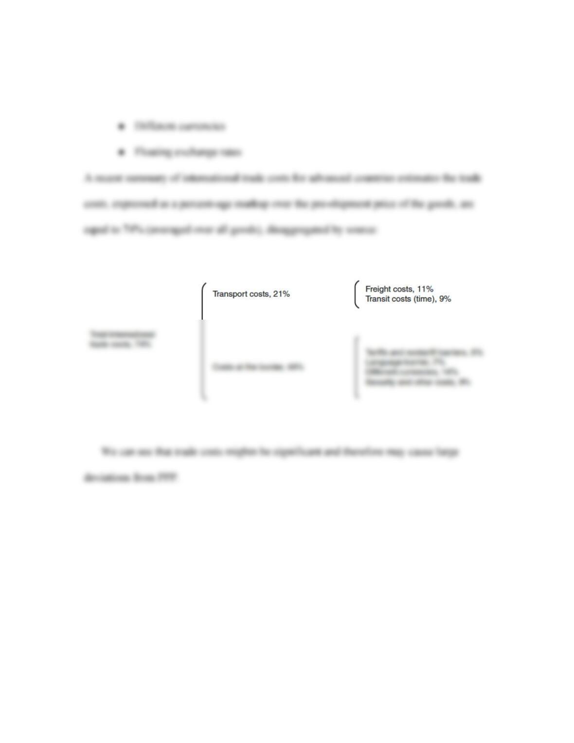
● Distance between markets
● Crossing international borders
APPLICATION
It’s Not Just the Burgers That Are Cheap
Trade costs imply that the real exchange rate will not equal 1. This application examines
the size of these deviations using The Economist’s Big Mac Index.
■ Deviations in PPP are not random.
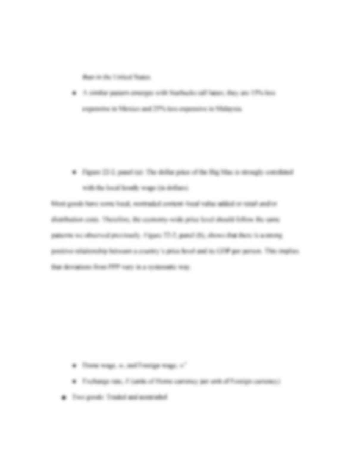
● Big Macs tend to be cheaper in poorer countries.
● Using 2010 data, Big Macs are 30% less in Mexico and 39% less in Malaysia
■ This can be explained by the existence of nontraded goods.
● The Big Mac is produced using a combination of traded goods (flour, beef,
and special sauce) and nontraded goods (cooks, cleaners, etc.).
Nontraded Goods and the Balassa‒Samuelson Model
This section outlines a model with two goods: one traded and the other nontraded. An
overview of the model follows:
■ Two countries: Home and Foreign
● Both goods are produced in competitive markets and labor is the only input
used.
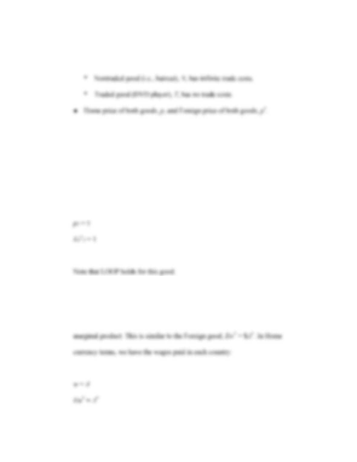
A Simple Model Solve the model in three steps:
1. The traded good has the same price in both countries. Because these goods have
no trade costs, they should sell for the same price in both countries. Prices are
denoted:
2. Productivity in traded goods determines wages. Each worker can produce A units
of the traded good per hour. The worker’s wage will be equal to $A (since the
price of the good is $1). Competition implies that each worker is paid his or her
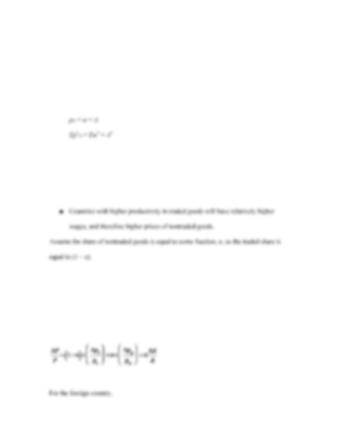
3. Wages determine the prices of nontraded goods. Each worker can produce one
unit of the nontraded good per hour. Competition means that the dollar price of a
good is equal to the wage paid (the marginal cost). Therefore,
The model has the following implications:
■ The overall price level in the economy depends on the share of nontraded goods
in the consumption basket and on the productivity in traded goods.
Changes in Productivity Home productivity increases (A rises). The change in the price
level is calculated as the weighted average of the change in prices in traded and
nontraded goods:
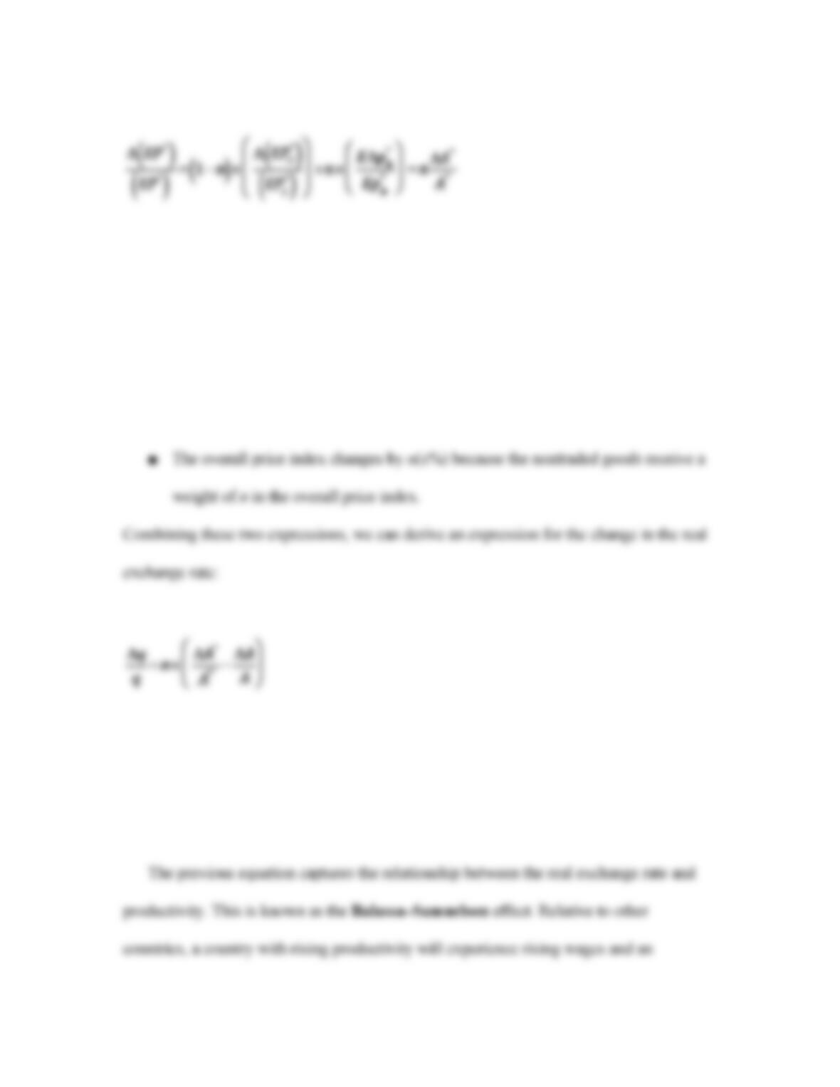
Changes in productivity affect the overall price index:
■ When the productivity of traded good increases by x%, wages must increase by
the same percentage.
■ The nontraded goods price will rise by the same x% because the price of the
nontraded good is equal to the wage.
Generalizing A country has relatively low wages because it has relatively low
productivity in the production of traded goods. This low productivity keeps the price of
nontraded goods and the overall price index low.
appreciation in the real exchange rate, meaning its price level is rising.
Overvaluations, Undervaluations, and Productivity Growth: Forecasting
Implications for Real and Nominal Exchange Rates
The Balassa‒Samuelson effect tells us that overall price levels should be higher in richer
countries. This is shown in Figure 22-3. In the figure, the line that best fits the data (a
regression line) is the predicted real exchange rate, . We observe that the actual data do
Forecasting the Real Exchange Rate Forecasting the real exchange rate, q can be
broken down into two problems:
■ How quickly q will return to its equilibrium value,
Convergence Empirical estimates suggest the half-life of deviations from PPP is five
years. In this example, after five years, the real exchange rate will increase by half of the
Convergence + Trend We can now calculate the implied change in the real exchange
rate. Convergence will cause the real exchange rate (q) to increase 2% each year. The
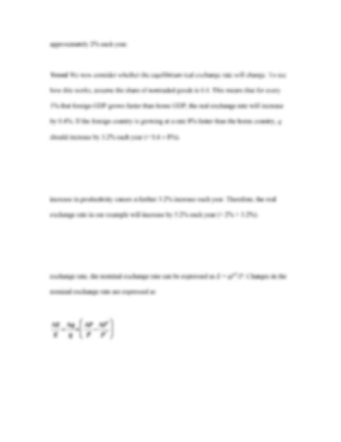
Forecasting the Nominal Exchange Rate If we are able to forecast the real exchange
rate, this will help forecast the nominal exchange rate. From the definition of the real
When relative PPP holds, the changes in the nominal exchange rate reflect inflation
differentials between home and foreign countries. When the Balassa‒Samuelson effect is
Adjustment to Equilibrium The previous expression shows us that changes in the
nominal exchange rate occur because of:
■ the Balassa–Samuelson effect—changes in the real exchange rate stemming from
convergence of q to the equilibrium real exchange rate, ,
■ Real undervaluation—home goods will become more expensive.
● Home goods’ prices must increase, or
APPLICATION
Real Exchange Rates in Emerging Markets
Here, we apply the previous model to study the behavior of the exchange rates relative to
the U.S. dollar. The data are from Figure 22-3.
China: Yuan Undervaluation?
■ Chinese yuan, 2000
● Balassa‒Samuelson model prediction: = 0.319
● Actual real exchange rate: q = 0.231
● Yuan–dollar exchange rate peg
■ What will happen to the real exchange rate?
● Trend: China’s growth rate exceeds that of the United States by 6%, implying
a further real appreciation of 2.4% per year (= 0.4 × 6, assuming 0.4 of goods
■ Forecasting the nominal exchange rate
● Nominal appreciation of yuan or increase in China’s inflation rate
Argentina: Was the Peso Overvalued?
■ Argentine peso, 2000
■ What will happen to the real exchange rate?
● Model predicts Argentina will experience a 22% real depreciation to close the
■ What did happen?
● To maintain the peg, Argentina’s prices must decrease relative to the United
Slovakia: Obeying the Rules?
■ Slovakian koruna in 2000
● Planned to join the EU and eventually the Eurozone. This required
maintenance of a managed floating exchange rate against the euro.
● Slovakia will experience an 89% real appreciation to close the gap
(0.252/0.656). Using the half-life estimates, this implies a 7.5% real
appreciation per year.
■ Dilemma:
● Slovakia experienced real appreciation of 5% to 10% per year from 1992 to
2004.
Conclusion
In general, PPP does not hold. Prices of goods are not the same in all countries. Arbitrage
fails because of trade costs. The final stake in the heart of PPP is the Balassa‒Samuelson
theorem, which incorporates nontraded goods into the model. These effects mean that the