
CHAPTER 11
A Real Intertemporal Model with Investment
KEY IDEAS IN THIS CHAPTER
2. A competitive equilibrium in this model is characterized by a combination of output,
3. The model can be used to analyze the macroeconomic effects of various shocks to the
economy.
4. For example, the model predicts that a temporary increase in government purchases
NEW IN THE FOURTH EDITION
2. Updated charts and tables.
TEACHING GOALS
It is important to emphasize that the possibility of accumulating capital represents a
fundamental difference to an economy. In the previous chapter, average consumption
must equal per capita total output less per capita government spending. For a given
amount of government savings, aggregate private savings is fixed. One consumer may
only reallocate consumption across time if another consumer is willing to make the
complementary reallocation. Borrowing and lending can improve economic outcomes
Many students try to get by with rote memorization of a great many curve shifts and
laundry lists of the effects of specific disturbances. However, to really understand this
material, students must be able to work out the effects of disturbances on their own.
I therefore encourage students to put a good deal of effort into solving problems with the

Chapter 11: A Real Intertemporal Model with Investment
CLASSROOM DISCUSSION TOPICS
This material allows the students to explore some interesting issues related to
macroeconomic shocks and how they affect the economy, and the effects of government
policy. The first issue is the effect of government spending, and it is important to relate
this to the fiscal policy responses to the financial crisis. In Canada, as in the United
States, there was a large “stimulus” package, typically motivated by Keynesian economic
reasoning. The modelling approach in this chapter can be used to call this reasoning into
question. What is a multiplier? How big could it be? These are questions this model can
answer. Keynesian models rely on more than just sticky wages and prices—there are
implicit assumptions about Ricardian equivalence (or its absence), for example, that
should be discussed here.
OUTLINE
1. The Representative Consumer
a) Consumer Choices
i) Current Work–Leisure Decision
ii) Future Work–Leisure Decision
iii) Consumption–Savings Decision
b) Current Labour Supply
i) Current Real Wage Effects
c) Current Demand for Consumption Goods
i) Real Interest Rate Effects
2. The Representative Firm
a) Firm Choices
i) Current Production
ii) Future Production

Instructor’s Manual for Macroeconomics, Fourth Canadian Edition
iii) Investment and Capital
iv) Depreciation of Capital
b) Profits and Current Labour Demand
i) Current Profits
ii) Future Profits
iii) The Present Value of Profits
iv) Current Employment Choice
c) The Investment Decision
i) The Marginal Cost of Investment
ii) The Marginal Benefit of Investment
iii) The Net Marginal Product of Capital
3. Government
a) Debt Issue
b) The Government’s Present-Value Budget Constraint
4. Competitive Equilibrium
a) The Current Labour Market and the Output Supply Curve
i) Slope of Output Supply—Real Interest Rate Effects
ii) Shifts in Output Supply
(2) Current Total Factor Productivity
(3) Current Capital Stock
b) The Current Goods Market and the Output Demand Curve
i) Slope of Output Demand—Real Interest Rate Effects
ii) Shifts in Output Demand
(2) The Present Value of Taxes
(4) Future Total Factor Productivity
c) The Complete Real Intertemporal Model
i) Equilibrium in the Goods Market
ii) Equilibrium in the Labour Market
5. A Temporary Increase in Government Purchases
a) Impact Effects
i) Labour Supply
ii) Output Supply
iii) Output Demand

6. A Reduction in the Current Capital Stock
a) Impact Effects
i) Labour Supply
ii) Labour Demand
iii) Output Supply
iv) Output Demand
b) Equilibrium Effects
i) Goods Market ?,Yr↓
ii) Labour Market ?,
N
w↓
7. An Increase in Current Total Factor Productivity
a) Impact Effects
i) Labour Supply
ii) Labour Demand
iii) Output Supply
b) Equilibrium Effects
i) Goods Market: ,Yr↑↓
ii) Labour Market ?(likely increases),
N
w↑
8. An Increase in Future Total Factor Productivity
a) Impact Effects
i) Labour Supply
ii) Output Demand
b) Equilibrium Effects
i) Goods Market: ,Yr↑↑
N
10. An Increase in Credit Market Uncertainty
a) Equilibrium Effects.
b) Interpretation in Terms of the Financial Crisis
Instructor’s Manual for Macroeconomics, Fourth Canadian Edition
TEXTBOOK QUESTION SOLUTIONS
Problems
1. There are two effects of an increase in the depreciation rate. First, there is the direct
effect, which implies that, given the marginal product of capital in period two,
,
K
M
P′the net marginal product of capital, ,
K
M
Pd
′−will decrease when the depreciation
rate increases. For any given real interest rate, this effect lowers investment demand,
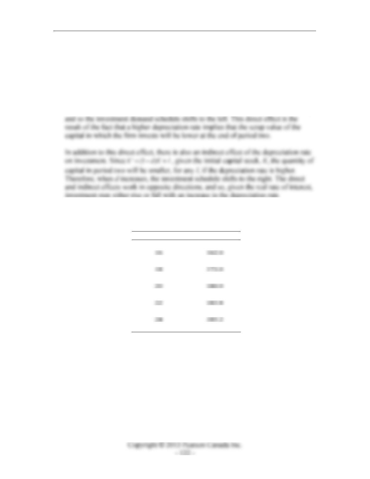
2. The problem supplies the following production function, where future output only
depends on the level of second-period capital, in this case the number of trees.
Future Trees Future Output
15 155.0
17 168.0
19 177.0
21 182.0
23 184.8
25 185.4
Chapter 11: A Real Intertemporal Model with Investment
a) The production function is depicted in Figure 11.1.
Figure 11.1
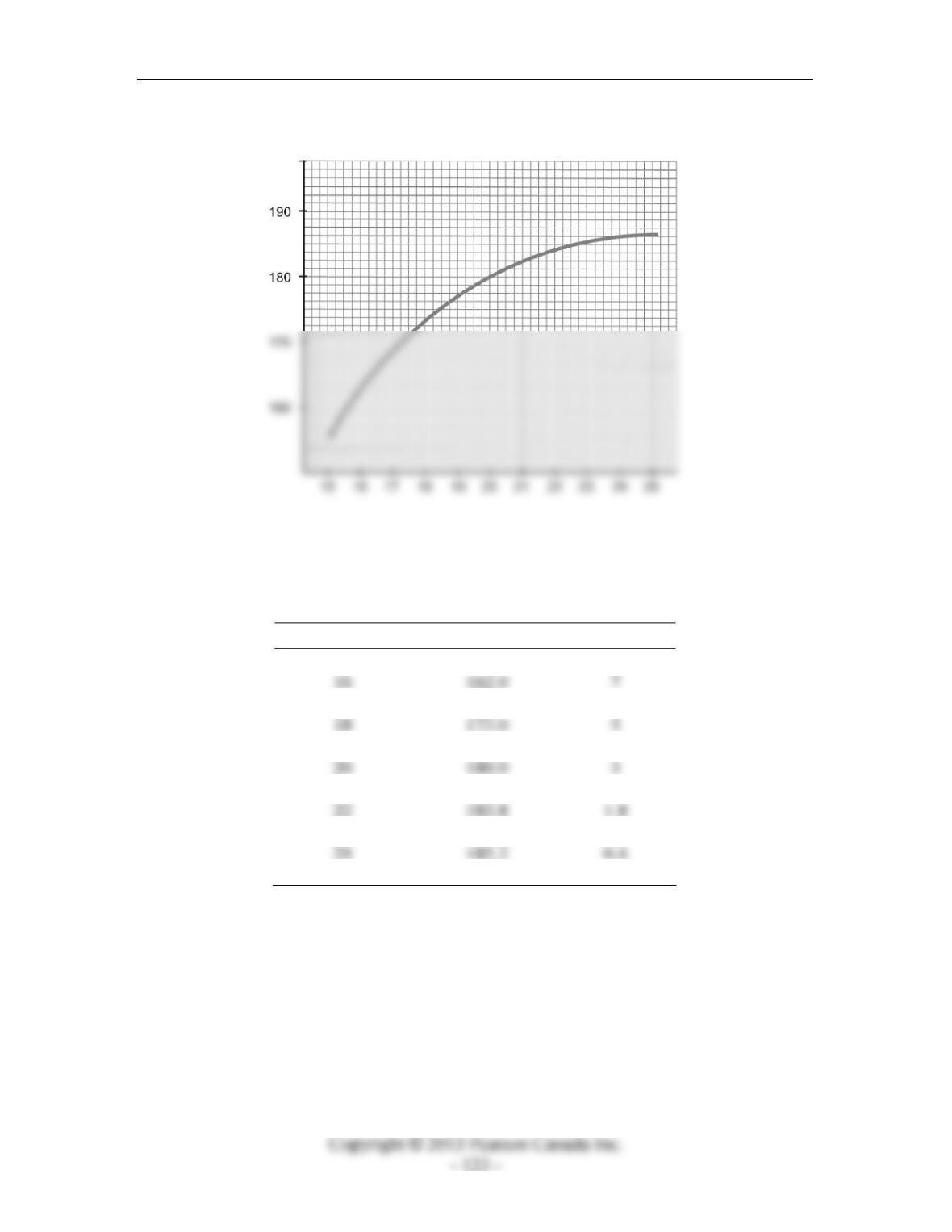
b) The marginal product of capital schedule is computed from the previous table. In
table form:
Future Trees Future Output ′
K
MP
15 155.0 –
17 168.0 6
19 177.0 4
21 182.0 2
23 184.8 1.0
25 185.4 0.2
These data are plotted in Figure 11.2.
Instructor’s Manual for Macroeconomics, Fourth Canadian Edition
Figure 11.2
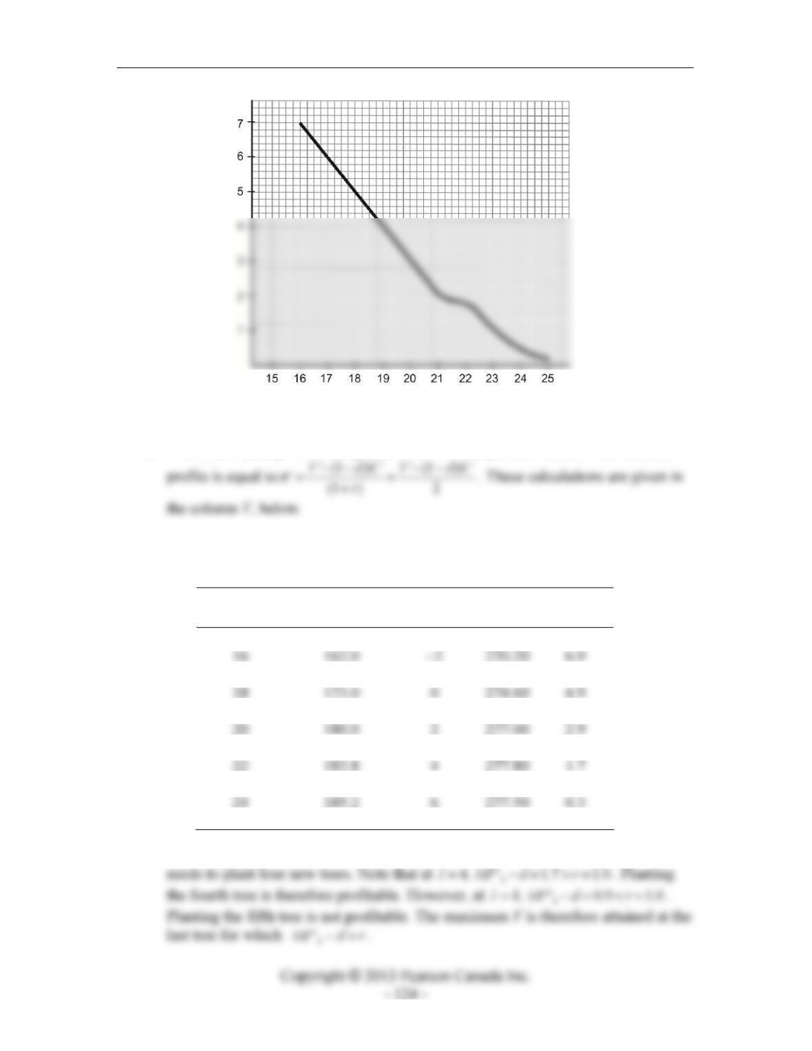
c) Tom’s first-year profits are equal to YI
π
=−. The present value of second-year
d) The net marginal product of capital is equal to 0.1
KK
MP d MP
′′
−= − These
calculations are also included in the table below.
Future Trees
Future
Output
Required I
V
′
K
MP d−
15 155.0 –3 267.25 –
17 168.0 –1 279.65 5.9
19 177.0 1 276.05 3.9
21 182.0 3 277.45 1.9
23 184.8 5 277.75 0.9
25 185.4 7 276.95 0.1
e) Tom’s optimal level of V is equal to 277.80. To earn this amount of profit, Tom
3. The costs of the output subsidy and the investment subsidy would each require an
increase in other (lump-sum) taxes to satisfy the government budget constraint with
unchanged government purchases. This increase in taxes reduces consumer wealth
and so labour supply shifts to the right and output supply also shifts to the right. This
effect tends to increase output and decrease the real interest rate.
In the case of the output subsidy, the decrease in the real interest rate increases both
consumption spending and investment spending to match the increase in output. In
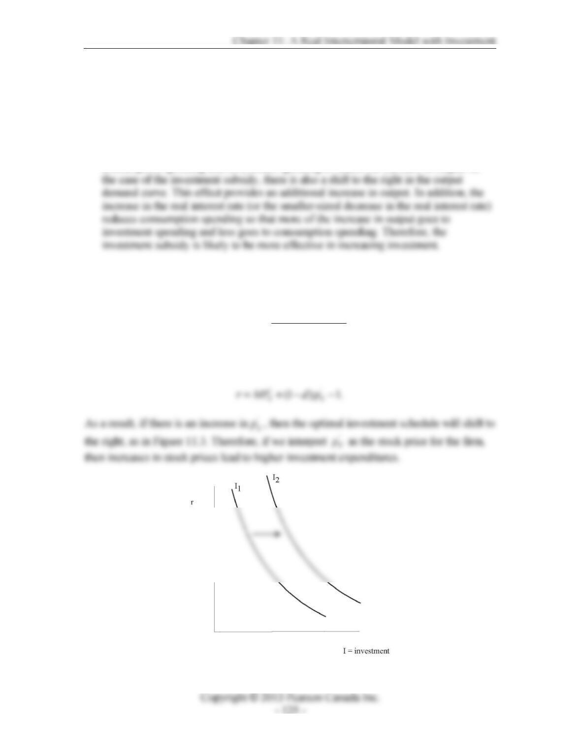
4. If capital can be sold at the end of the future period at the price ‘
K
p
, then the marginal
cost of investment is still 1, but the marginal benefit of investment is given by
”
(1 )
() 1
K
K
M
Pdp
MB I r
+−
=+.
The firm invests to the point where the marginal cost of investment is equal to the
marginal benefit, which gives the optimal investment rule
K
Figure 11.3

5. Slope of the output demand curve.
a) A reduction in the real interest rate increases consumption and investment
spending. This is the primary reason for the downward slope of the output
demand curve. However, as output rises, there is a further increase in
6. Slope of the output supply curve.
a) Figure 11.4 depicts the effect of an increase in labour supply, due to an increase in
the real interest rate, on the equilibrium level of employment. The diagram shows
two alternate labour demand curves with differing slopes. Note that the

Chapter 11: A Real Intertemporal Model with Investment
Figure 11.4
b) When the substitution effect of an increase in the real rate of interest decreases, an
7. For part (a), this has no effect, due to Ricardian equivalence. The multiplier is zero.
For part (b), the output demand curve shifts to the right, as some consumers
8. Labour supply shifts to the right, so output supply also shifts to the right.
Consumption demand also increases, so the output demand curve must also shift to
the right. Output must increase although the real rate of interest may rise or fall. In
light of the increase in output, equilibrium employment must increase. A higher level

Instructor’s Manual for Macroeconomics, Fourth Canadian Edition
9. A temporary increase in z increases output and employment, raises the real wage, and
lowers the real rate of interest. Consumption and investment both increase. An
increase in future total factor productivity, z’, shifts the current-period output demand
curve to the right. Current output and employment increase, and the real interest rate
increases. Since the current-period labour demand curve does not shift, the shift in
labour supply due to the lower real interest rate causes the real wage rate to decline.
A permanent increase in total factor productivity simply combines the effects of the
10. The increase in z’ shifts the output demand curve to the right, but has no effect on the
output supply curve. The increase in K shifts the output demand curve to the left, and
shifts the output supply curve to the right. The combined effects shift the output
supply curve to the right. The shift in the output demand curve is uncertain. An
increase in the current capital stock lowers investment spending. An increase in future
total factor productivity increases investment spending. As one possibility, suppose
that the effect of the prospective increase in total factor productivity is that investment
increases. In this case, both the output supply curve and the output demand curve shift
to the right. Output rises unambiguously, but the effect on the real interest rate is
uncertain.
If a lack of capital were the only reason for low output in poor countries, then we
11. A temporary increase in the price of energy is best modelled as a reduction in current-
period total factor productivity. Such a disturbance shifts output supply to the left.
Therefore, output falls and the real interest rate increases. In question 4, above, we
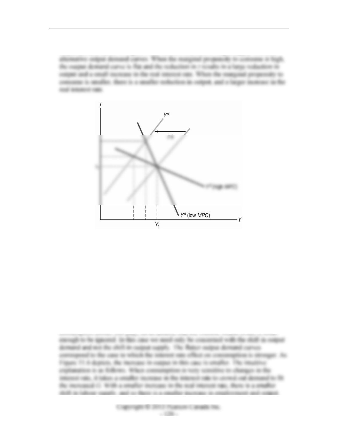
Chapter 11: A Real Intertemporal Model with Investment
showed that a larger value for the marginal propensity to consume implied a flatter
output demand curve. In Figure 11.5, we show the shift in output supply with two
Figure 11.5
12. A short war is best modelled as a temporary increase in government spending. Such a
disturbance shifts the output demand curve to the right because the increase in
current-period government spending will be larger than the reduction in consumption
demand due to the decline in consumers’ lifetime wealth. The output supply curve
also shifts to the right because of the reduction in consumers’ lifetime wealth. Output
and employment unambiguously increase. Because the increase in government
spending is only temporary, the effect on lifetime wealth is likely to be small, so the
demand curve shifts farther than the supply curve. Therefore, the interest rate most
likely increases.
In order to see more clearly how the size of the intertemporal substitution effect on
consumption comes into play, let us assume that the lifetime wealth effect is small
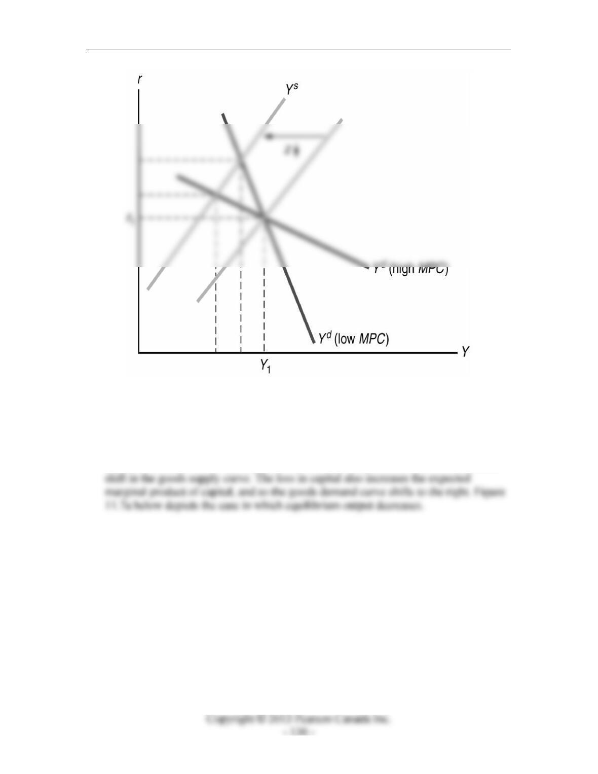
Instructor’s Manual for Macroeconomics, Fourth Canadian Edition
Figure 11.6
13. A hurricane destroys a significant amount of capital. This disturbance may be
analyzed as an exogenous decrease in the stock of capital. The production function
shifts downward. Labour demand shifts to the left. These effects result in a leftward
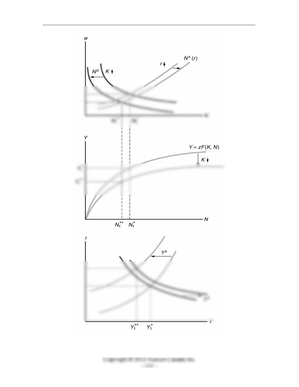
Chapter 11: A Real Intertemporal Model with Investment
Figure 11.7a
Instructor’s Manual for Macroeconomics, Fourth Canadian Edition
a) The analysis of the effects of the hurricane suggests that it is reasonable to expect
a decrease in national income. However, because the model is based upon
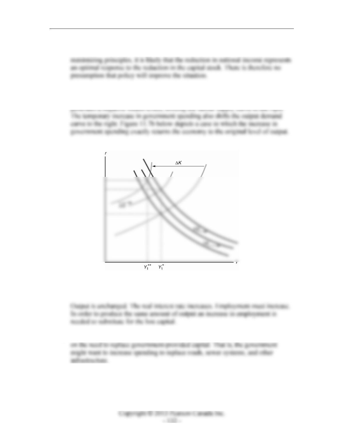
b) An appropriate-sized increase in government spending can restore the economy to
the original level of output *
1
Y. A temporary increase in government spending
Figure 11.7b
c) A more sensible rationale for an increase in government spending would be based
14. For this question, simply put together Figure 11.26 with Figure 11.21 from the
text. The increase in credit market risk acts to reduce equilibrium aggregate
output, and the appropriate increase in G will be just enough to offset this and
leave output unchanged. The model certainly does not give us a rationale for this