Basic Econometrics, Gujarati and Porter
127
CHAPER 11:
HETEROSCEDASTICITY: WHAT HAPPENS WHEN ERROR
VARIANCE IS NONCONSTANT?
11.1 (a) False. The estimators are unbiased but are inefficient.
11.2 (a) As equation (1) shows, as N increases by a unit, on average,
(b) Apparently, the author was concerned about heteroscedasticity,
11.3 (a) No. These models are non-linear in the parameters and cannot be
128
(c) Let
1 2
ln ln ln
i i i
Y X u
β β
= + +
11.6
(a)The assumption made is that the error variance is proportional to
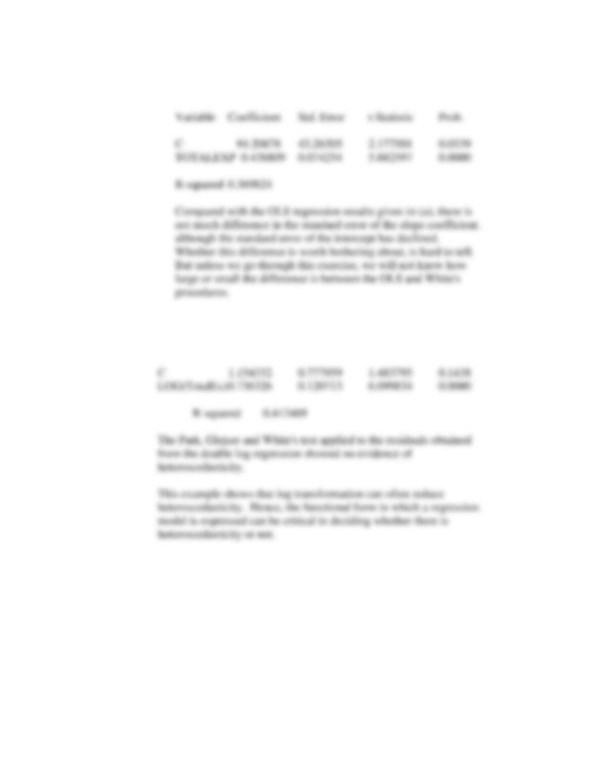
(b) The results are essentially the same, although the standard errors
11.7
As will be seen in Problem 11.13, the Bartlett test shows that there
11.8
Substituting w
w in (11.3.8), we obtain:
11.9 From Eq. (11.2.2), we have
Basic Econometrics, Gujarati and Porter
Empirical Exercises
11.11 The regression results are already given in (11.5.3). If average
productivity increases by a dollar, on average, compensation
increases by about 23 cents.
(a) The residuals from this regression are as follows:
(c) The regression results are:
Basic Econometrics, Gujarati and Porter
(d) If you rank the absolute residuals from low to high value
and similarly rank average productivity figures from low to high
11.12 (a) & (b)
(c) The regression results are:
6.8
7.2
7.8
0.2 0.4 0.6 0.8 1.0
Basic Econometrics, Gujarati and Porter
131
11.14 Using the formula (11.3.8) for weighted least-squares, it can be
shown that
11.15
(a) The regression results are as follows:
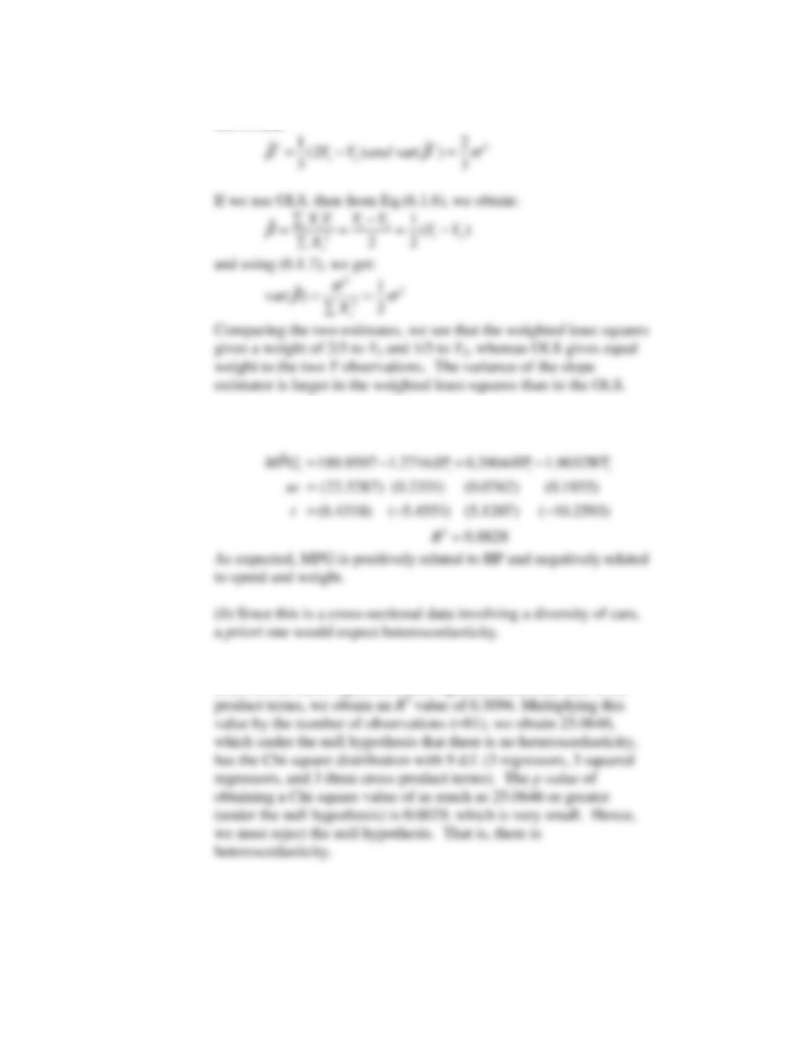
(c) Regressing the squared residuals obtained from the model shown
in (a) on the three regressors, their squared terms, and their cross-
Basic Econometrics, Gujarati and Porter
132
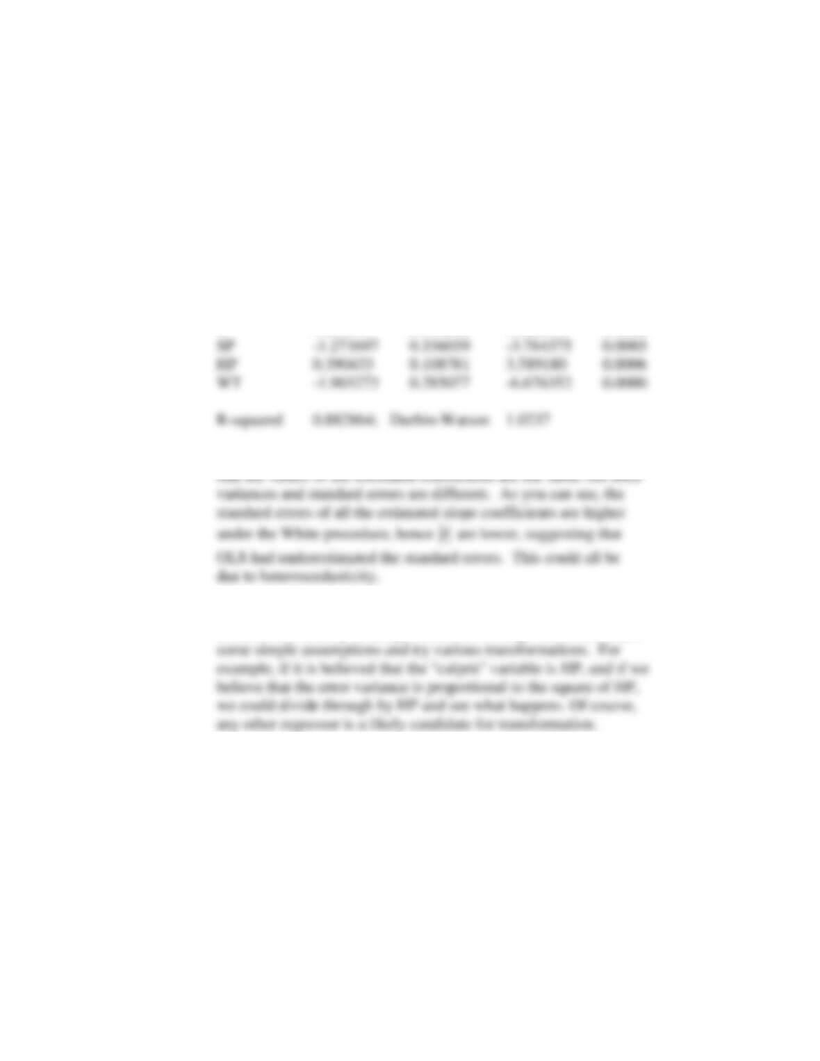
(d)The results based on White’s procedure are as follows:
Dependent Variable: MPG
Method: Least Squares
Sample: 1 81
Included observations: 81
White Heteroscedasticity-Consistent Standard Errors & Covariance
Variable Coefficient Std. Error t-Statistic Prob.
C 189.9597 33.90605 5.602531 0.0000
When you compare these results with the OLS results, you will find
(e)
There is no simple formula to determine the exact nature
of heteroscedasticity in the present case. Perhaps one could make
11.16
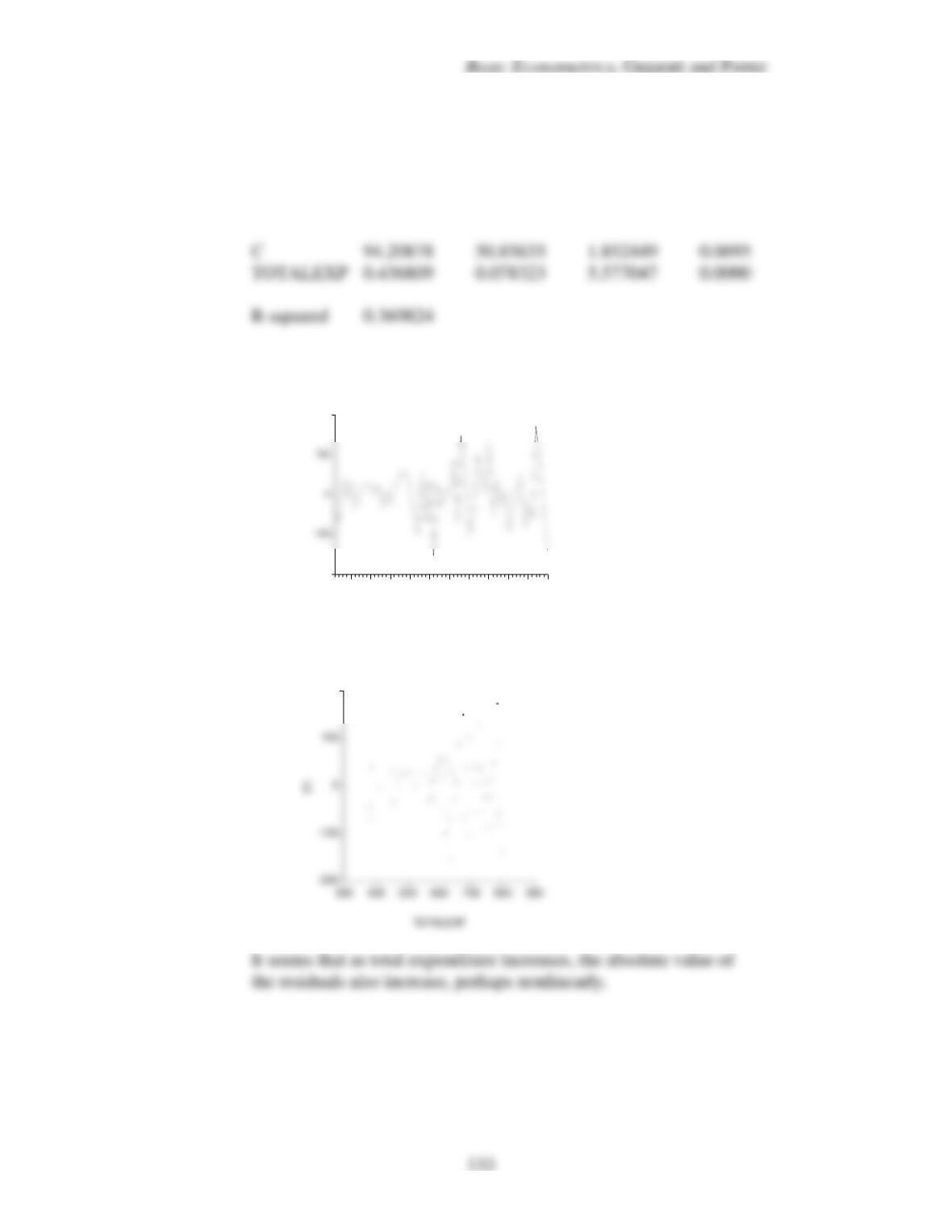
(a) The regression results are as follows:
Dependent Variable: FOODEXP
Variable Coefficient Std. Error t-Statistic Prob.
The residuals obtained from this regression look as follows:
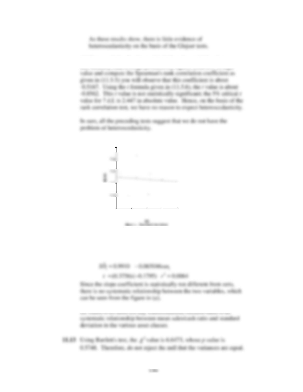
(b) Plotting residuals (R1) against total expenditure, we observe
–200
200
5 10 15 20 25 30 35 40 45 50 55
200
Basic Econometrics, Gujarati and Porter
134
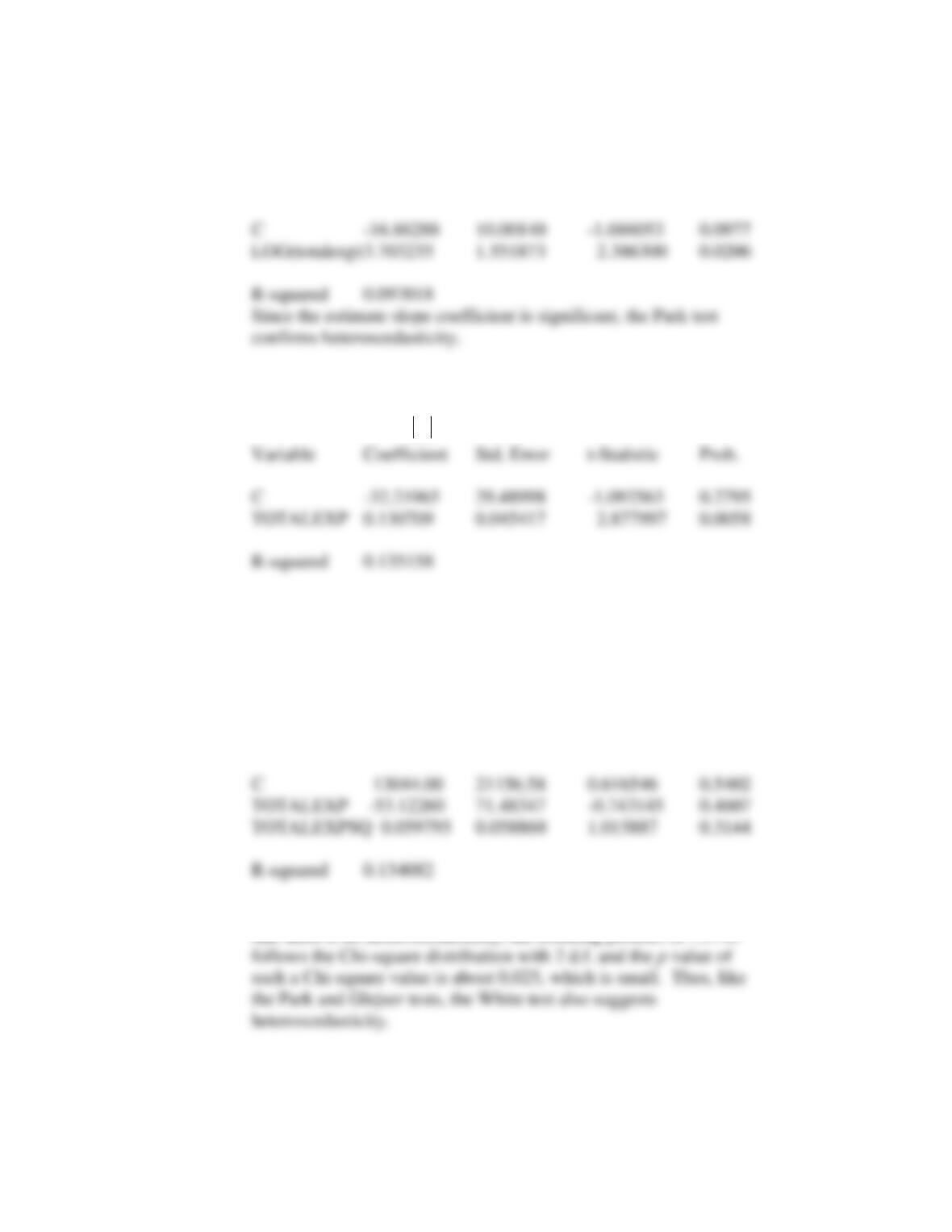
(c)Park Test
Dependent Variable: LOG (RESQ)
Variable Coefficient Std. Error t-Statistic Prob.
Glejser Test
Dependent Variable:
ˆ
i
u
, absolute value of residuals
Since the estimated slope coefficient is statistically significant, the
Glejser test also suggests heteroscedasticity.
White Test
Dependent Variable:
2
ˆ
i
u
Variable Coefficient Std. Error t-Statistic Prob.
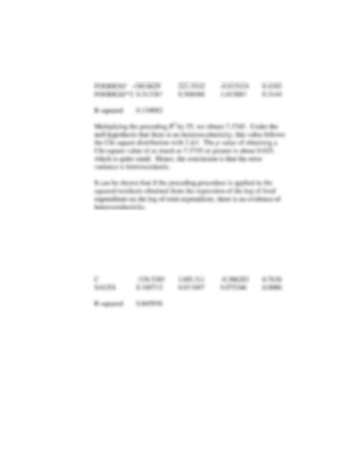
If you multiply the R-squared value by 55, and the null hypothesis is
that there is no heteroscedasticity, the resulting product of 7.3745
Basic Econometrics, Gujarati and Porter
135
(d)
The White heteroscedasticity-corrected results are as follows:
Dependent Variable: FOODEXP
11.17
The regression results are as follows:
Variable Coefficient Std. Error t-Statistic Prob.
11.18
The squared residuals from the regression of food expenditure
on total expenditure were first obtained, denoted by R
12
.Then they
were regressed on the forecast and forecast squared value obtained
from the regression of food expenditure on total expenditure. The
results were as follows:
Basic Econometrics, Gujarati and Porter
136
Dependent Variable:R
12
Variable Coefficient Std. Error t-Statistic Prob.
C 27282.63 39204.59 0.695904 0.4896
11.19
There is no reason to believe that the results will be any different
because profits and sales are highly correlated, as can be seen from
the following regression of profits on sales.
Dependent Variable: PROFITS
Variable Coefficient Std. Error t-Statistic Prob.
137
11.20
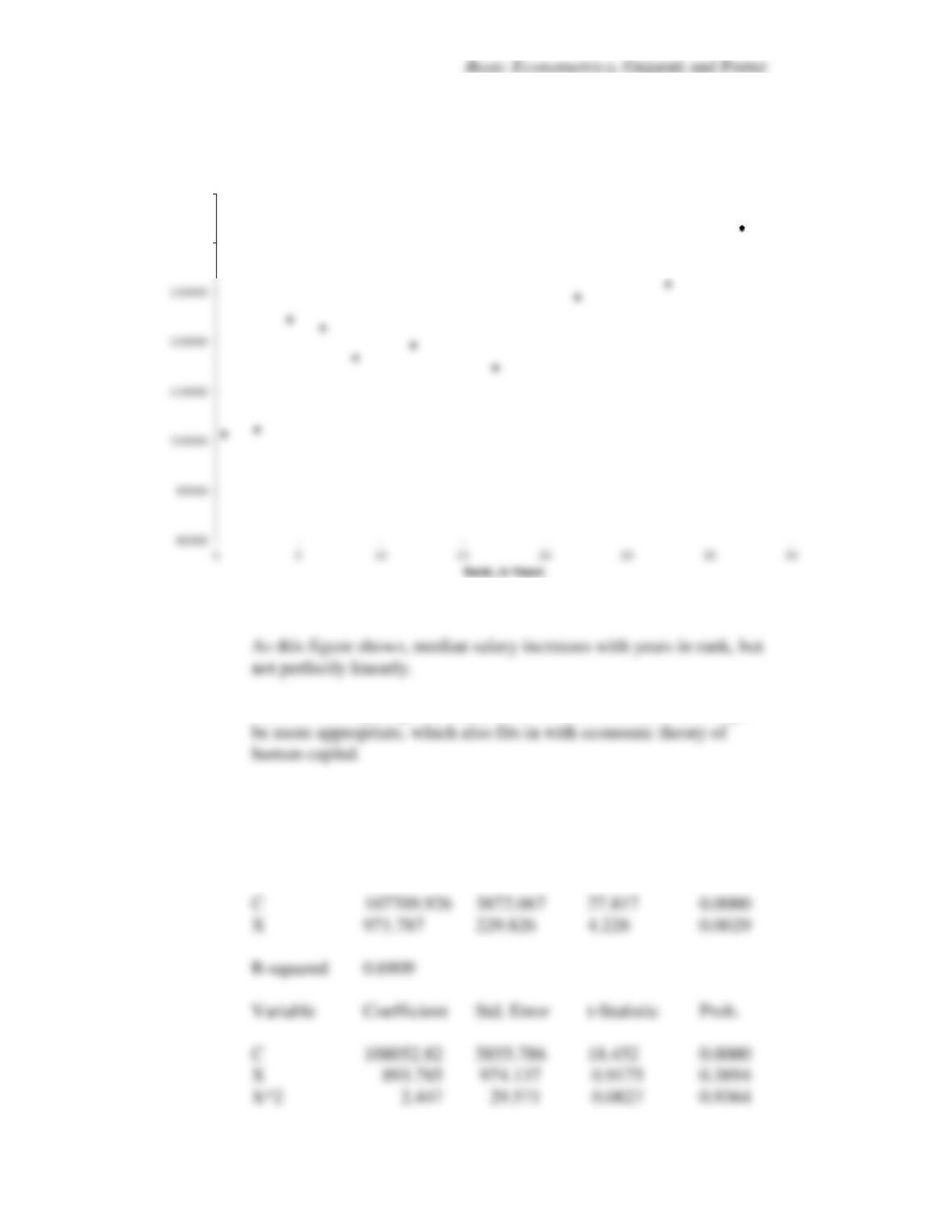
(a)
(b) From the figure given in (a) it would seem that model (2) might
(c) The results of fitting both the linear and quadratic models are as
follows:
Variable Coefficient Std. Error t-Statistic Prob.
Salaries vs Rank
140000
150000
Basic Econometrics, Gujarati and Porter
138
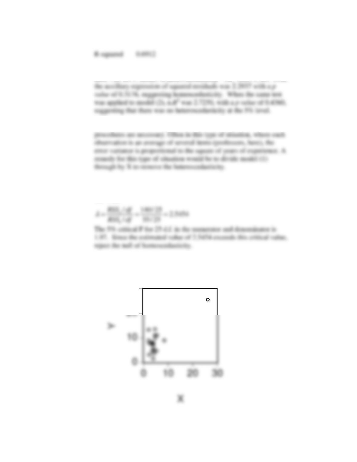
(c)White’s heteroscedasticity test applied to model (1) showed that
there was not evidence of heteroscedasticity. The value of n.R
2
from
(d) Since there was no apparent heteroscedasticity, no further
11.21
The calculated test statistic,
( )
F is
λ
=
11.22
(a) The graph is as follows.
30
Basic Econometrics, Gujarati and Porter
139
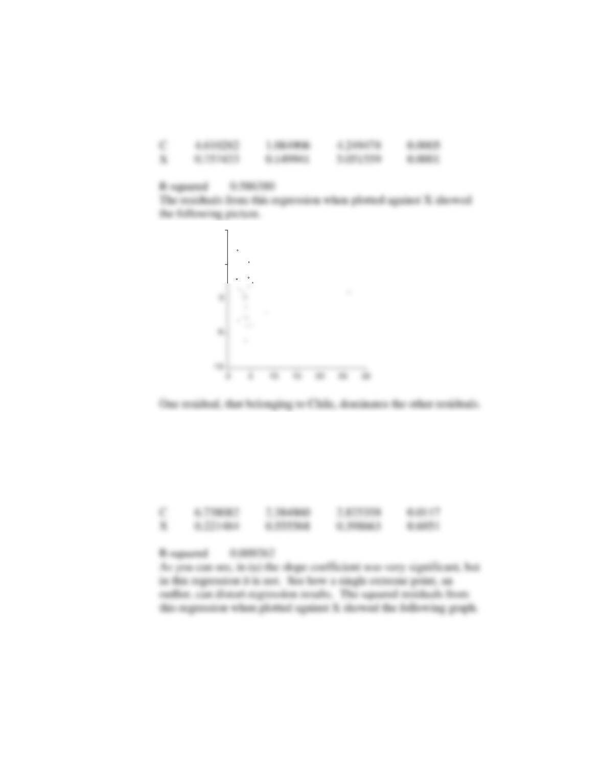
(b) The regression results are:
Variable Coefficient Std. Error t-Statistic Prob.
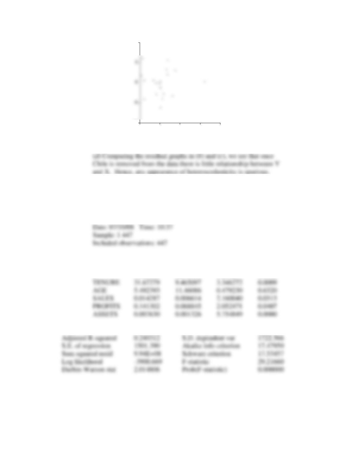
(c) Excluding the observation for Chile, the regression results were
as follows:
Variable Coefficient Std. Error t-Statistic Prob.
5
10
Basic Econometrics, Gujarati and Porter
140
11.23
(a) Regression results from EViews are as follows:
Dependent Variable: SALARY
Method: Least Squares
Variable Coefficient Std. Error t-Statistic Prob.
C 998.7095 623.6954 1.601277 0.1100
R-squared 0.248829 Mean dependent var 2027.517
-10
10
2 4 6 8 10
Basic Econometrics, Gujarati and Porter
141
The results for the White Heteroskedasticity test are:
White Heteroskedasticity Test:
(b) Results for the log-lin model and White’s heteroscedasticity test are as follows:
Dependent Variable: LN_SAL
Method: Least Squares
Date: 07/10/08 Time: 13:56
Sample: 1 447
Included observations: 447
Variable Coefficient Std. Error t-Statistic Prob.
C 6.753659 0.236823 28.51778 0.0000
R-squared 0.208984 Mean dependent var 7.391898
Adjusted R-squared 0.200016 S.D. dependent var 0.637388
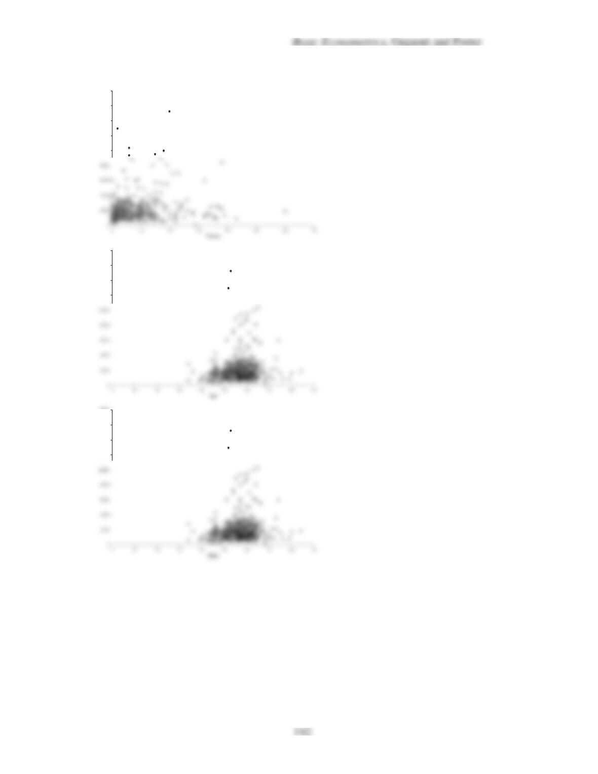
(c)
10000
12000
14000
16000
18000
12000
14000
16000
18000
12000
14000
16000
18000
Basic Econometrics, Gujarati and Porter
143
16000
18000
12000
14000
16000
18000