Questions for Review
1. The aggregate demand curve represents the negative relationship between the price
level and the level of national income. In Chapter 9, we looked at a simplified theory of
aggregate demand based on the quantity theory. In this chapter, we explore how the
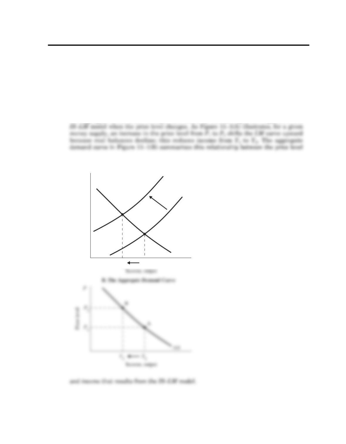
IS–LM model provides a more complete theory of aggregate demand. We can see why
the aggregate demand curve slopes downward by considering what happens in the
96
LM (P = P2)
Y2
LM (P = P1)
Y1
A. The IS LM Model
r
Interest rate
B
A
IS
–
Figure 11–1
CHAPTER 11 Aggregate Demand II
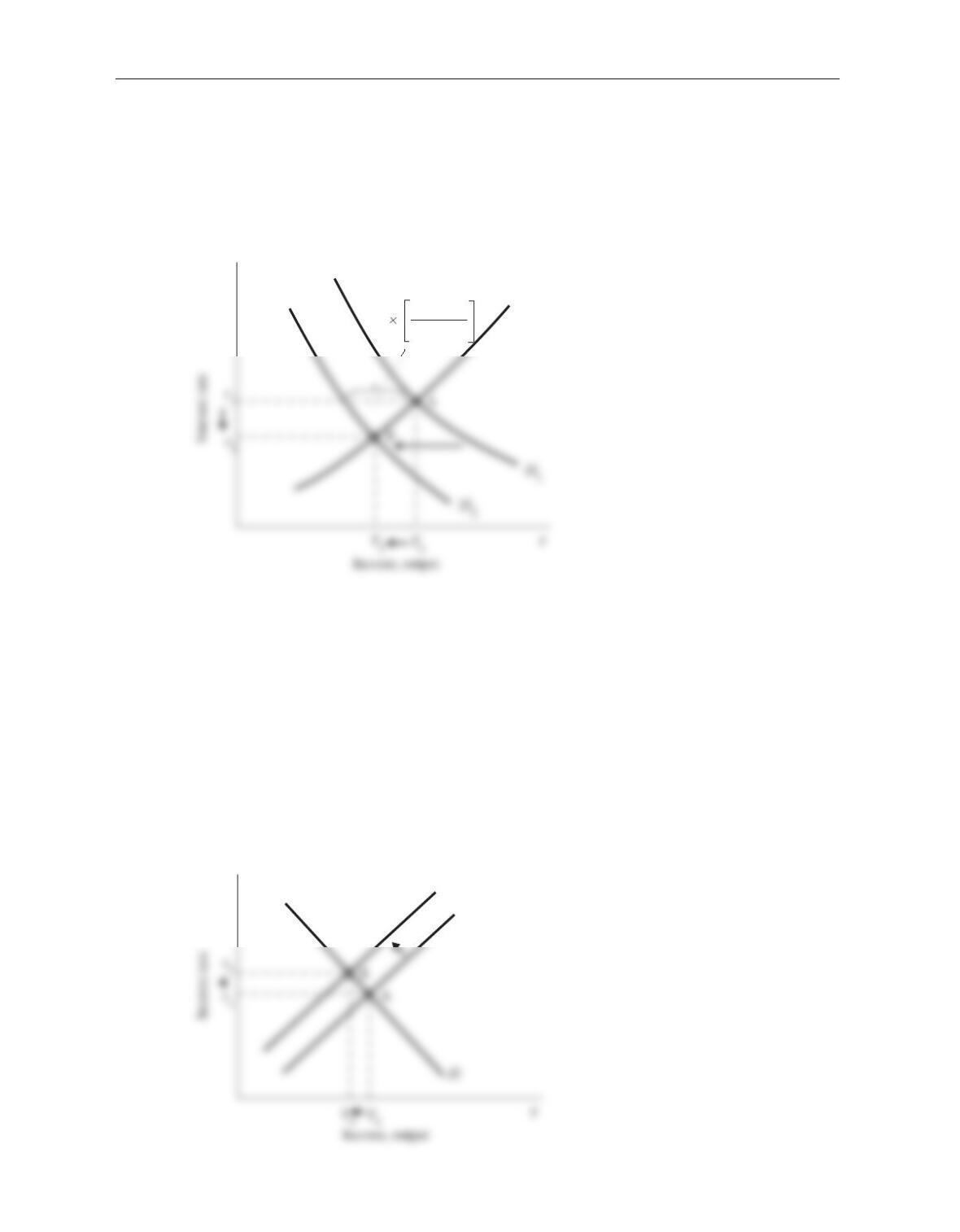
2. The tax multiplier in the Keynesian-cross model tells us that, for any given interest
rate, the tax increase causes income to fall by ΔT×[ – MPC/(1 – MPC)]. This IS curve
shifts to the left by this amount, as in Figure 11–2. The equilibrium of the economy
moves from point A to point B. The tax increase reduces the interest rate from r1to r2
and reduces national income from Y1to Y2. Consumption falls because disposable
income falls; investment rises because the interest rate falls.
Note that the decrease in income in the IS–LM model is smaller than in the
Keynesian cross, because the IS–LM model takes into account the fact that investment
rises when the interest rate falls.
3. Given a fixed price level, a decrease in the nominal money supply decreases real money
balances. The theory of liquidity preference shows that, for any given level of income, a
decrease in real money balances leads to a higher interest rate. Thus, the LM curve
shifts upward, as in Figure 11–3. The equilibrium moves from point A to point B. The
decrease in the money supply reduces income and raises the interest rate.
Consumption falls because disposable income falls, whereas investment falls because
the interest rate rises.
LM
r
Δ T 1 – MPC
– MPC
Figure 11–2
r
LM2
LM1
Figure 11–3
Chapter 11 Aggregate Demand II 97
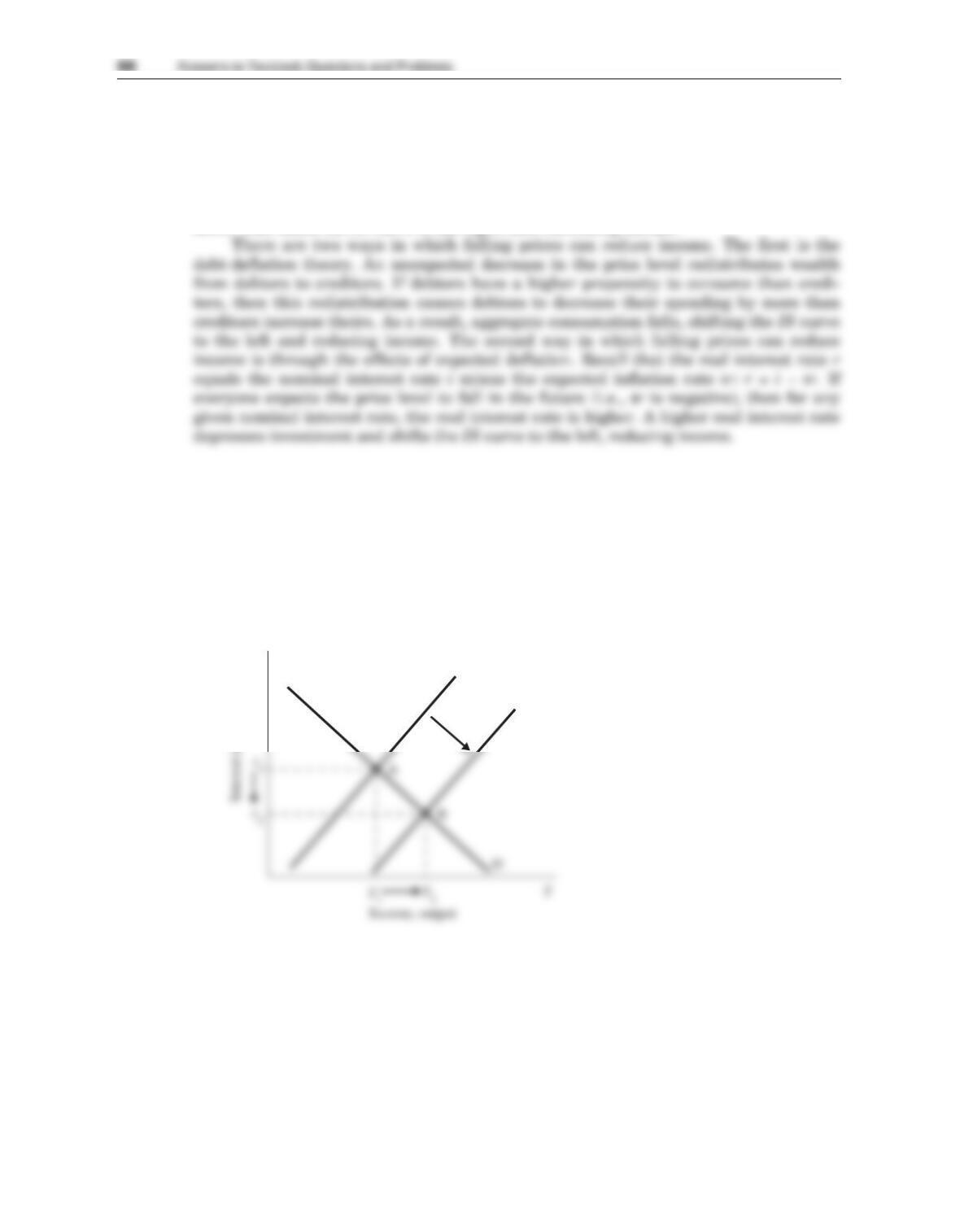
4. Falling prices can either increase or decrease equilibrium income. There are two ways
in which falling prices can increase income. First, an increase in real money balances
shifts the LM curve downward, thereby increasing income. Second, the IS curve shifts
to the right because of the Pigou effect: real money balances are part of household
wealth, so an increase in real money balances makes consumers feel wealthier and buy
more. This shifts the IS curve to the right, also increasing income.
Problems and Applications
1. a. If the central bank increases the money supply, then the LM curve shifts down-
ward, as shown in Figure 11–4. Income increases and the interest rate falls. The
increase in disposable income causes consumption to rise; the fall in the interest
rate causes investment to rise as well.
r
LM1
LM2
Figure 11–4
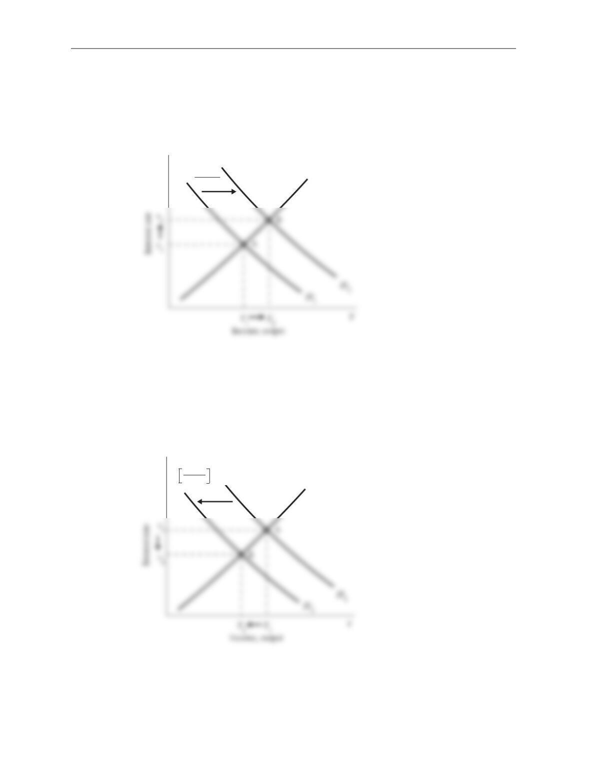
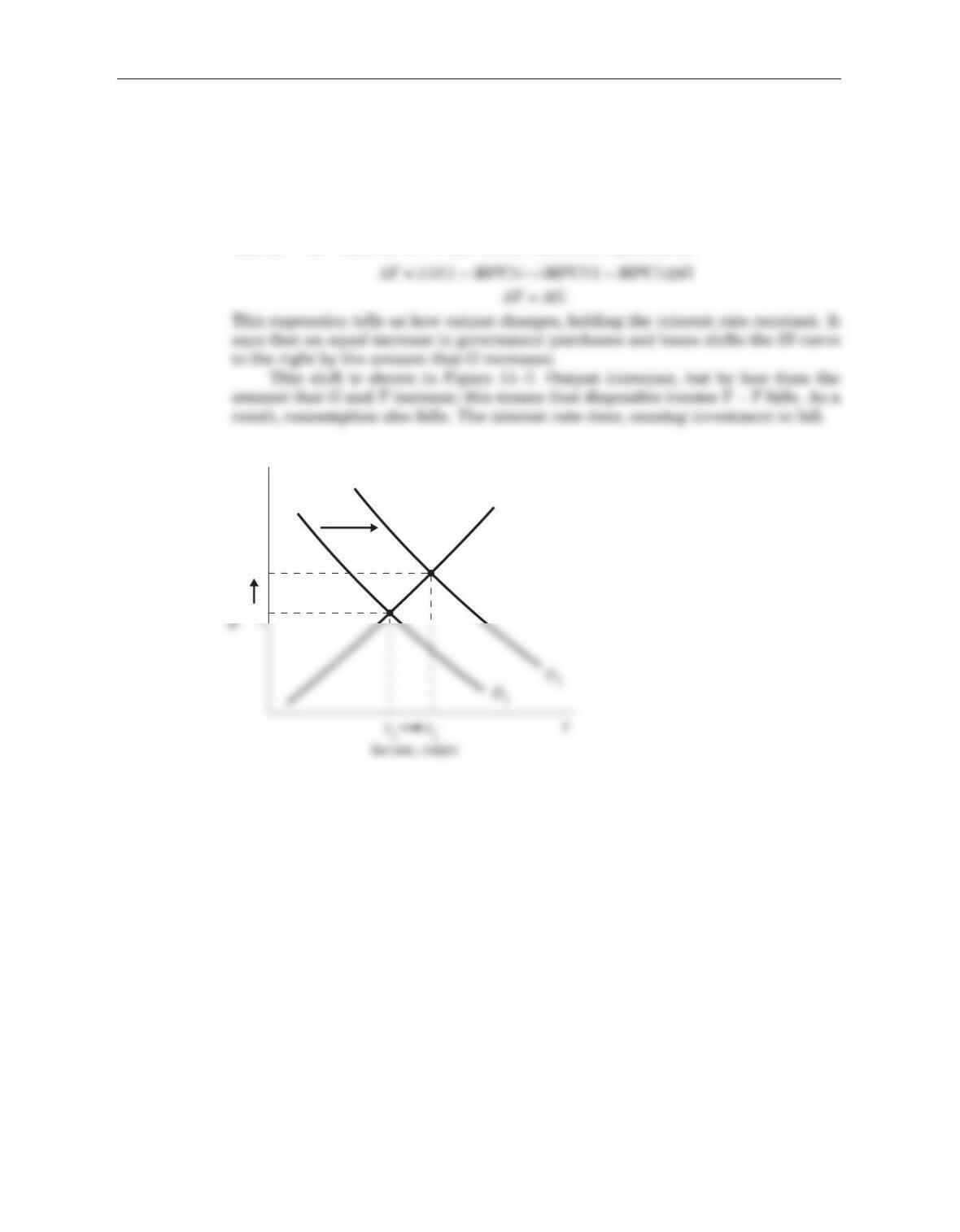
b. If government purchases increase, then the government-purchases multiplier tells
us that the IS curve shifts to the right by an amount equal to [1/(1 – MPC)]ΔG.
This is shown in Figure 11–5. Income and the interest rate both increase. The
increase in disposable income causes consumption to rise, while the increase in
the interest rate causes investment to fall.
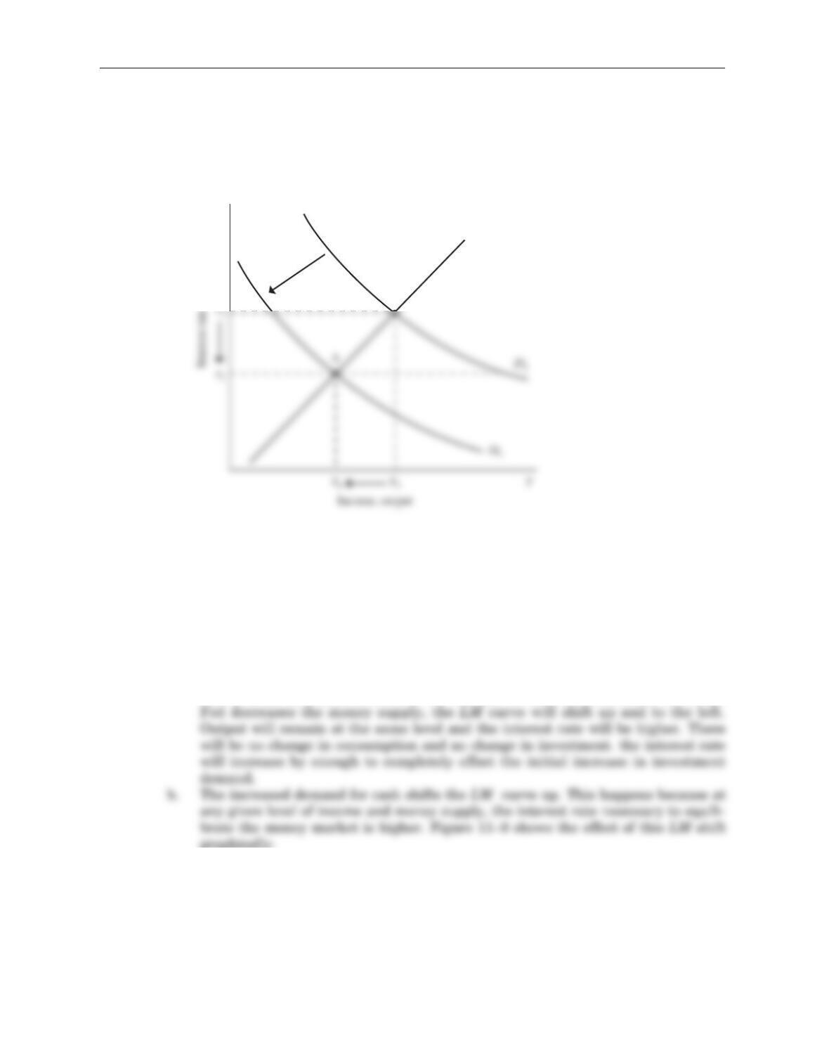
c. If the government increases taxes, then the tax multiplier tells us that the IS
curve shifts to the left by an amount equal to [ – MPC/(1 – MPC)]ΔT. This is
shown in Figure 11–6. Income and the interest rate both fall. Disposable income
falls because income is lower and taxes are higher; this causes consumption to
fall. The fall in the interest rate causes investment to rise.
Chapter 11 Aggregate Demand II 99
LM
Δ G
1 – MPC
r
Figure 11–5
LM
r
– MPC
1 – MPC Δ T
Figure 11–6
d. We can figure out how much the IS curve shifts in response to an equal increase
in government purchases and taxes by adding together the two multiplier effects
that we used in parts (b) and (c):
ΔY= [(1/(1 – MPC))]ΔG] – [(MPC/(1 – MPC))ΔT]
Because government purchases and taxes increase by the same amount, we know
that ΔG= ΔT. Therefore, we can rewrite the above equation as:
100 Answers to Textbook Questions and Problems
LM
B
A
r
ΔG
r2
r1
Figure 11–7
Chapter 11 Aggregate Demand II 101
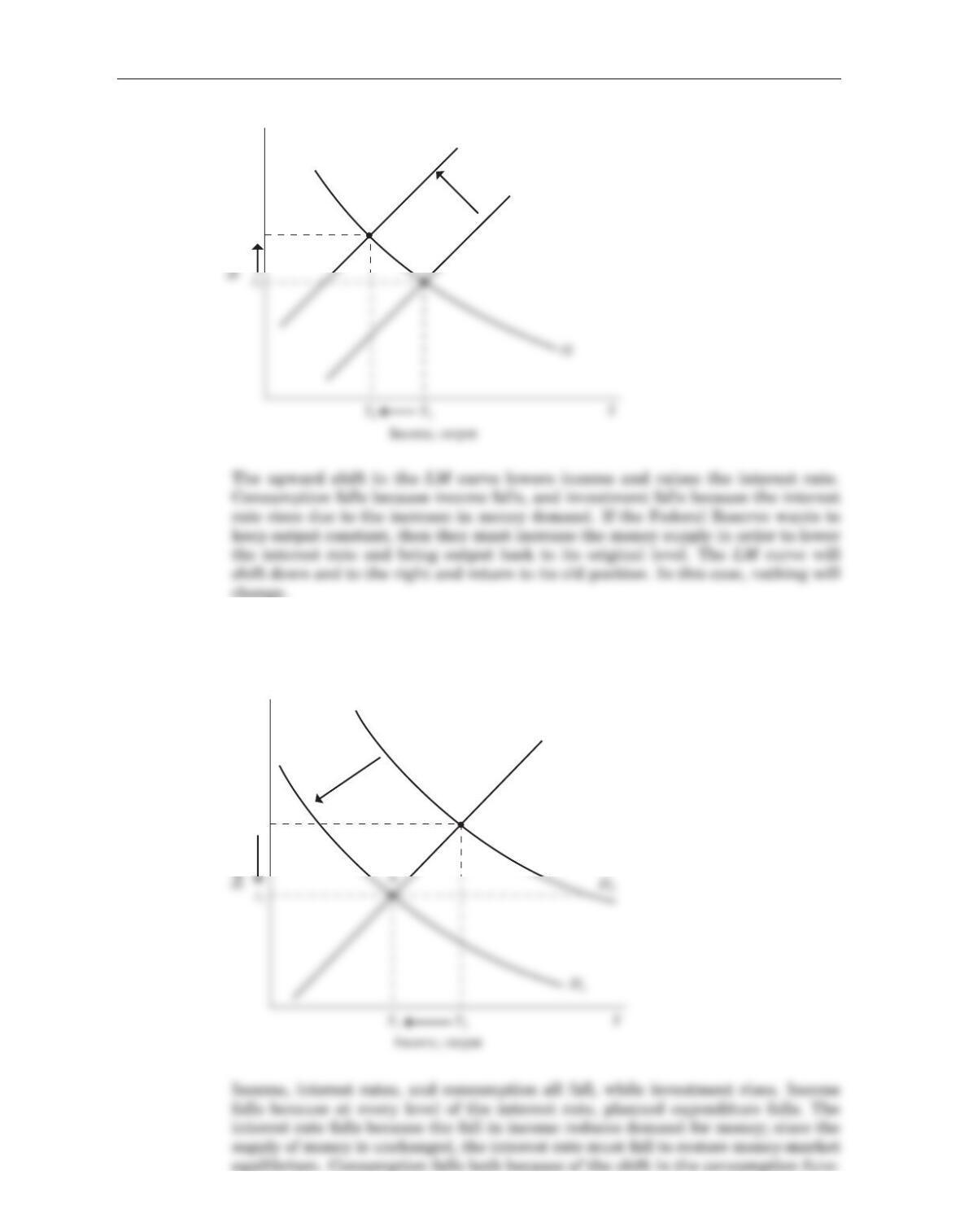
2. a. The invention of the new high-speed chip increases investment demand, meaning
that at every interest rate, firms want to invest more. The increase in the demand
for investment goods shifts the IS curve out and to the right, raising income and
employment. Figure 11–8 shows the effect graphically.
The increase in income from the higher investment demand also raises interest
rates. This happens because the higher income raises demand for money; since
the supply of money does not change, the interest rate must rise in order to
restore equilibrium in the money market. The rise in interest rates partially off-
sets the increase in investment demand, so that output does not rise by the full
amount of the rightward shift in the IS curve. Overall, income, interest rates, con-
sumption, and investment all rise. If the Federal Reserve wants to keep output
constant, then it must decrease the money supply and increase interest rates fur-
ther in order to offset the effect of the increase in investment demand. When the
B
LM
r
Figure 11–8
102 Answers to Textbook Questions and Problems
c. At any given level of income, consumers now wish to save more and consume less.
Because of this downward shift in the consumption function, the IS curve shifts
inward. Figure 11–10 shows the effect of this IS shift graphically.
B
LM
r
r2
Figure 11–10
B
r
r2
A
LM2
LM1
Figure 11–9
Chapter 11 Aggregate Demand II 103
tion and because income falls. Investment rises because of the lower interest rates
and partially offsets the effect on output of the fall in consumption. If the Federal
Reserve wants to keep output constant, then they must increase the money supply
in order to reduce the interest rate and increase output back to its original level.
The increase in the money supply will shift the LM curve down and to the right.
Output will remain at its original level, consumption will be lower, investment
will be higher, and interest rates will be lower.
3. a. The IS curve is given by:
Y= C(Y– T) + I(r) + G.
We can plug in the consumption and investment functions and values for Gand T
as given in the question and then rearrange to solve for the IS curve for this econ-
omy:
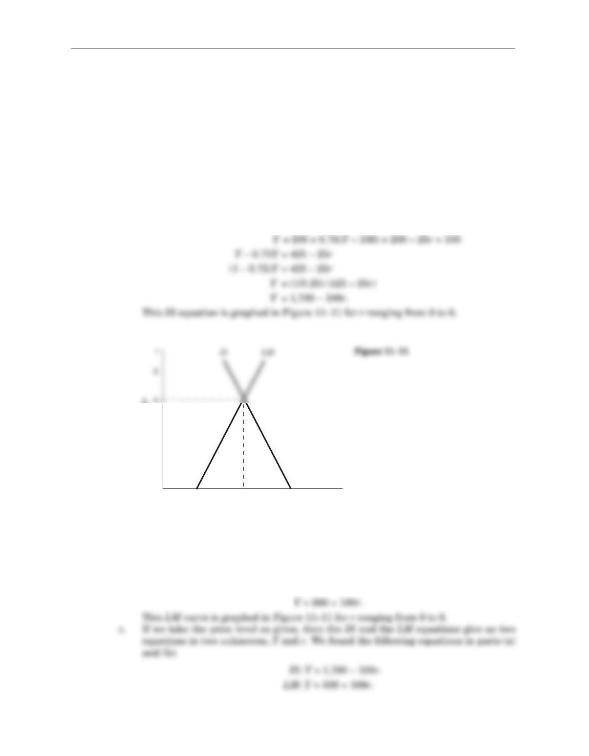
b. The LM curve is determined by equating the demand for and supply of real money
balances. The supply of real balances is 1,000/2 = 500. Setting this equal to money
demand, we find:
500 = Y– 100r.
Y
1,7001,100500
0
Interest rate
Income, output

Equating these, we can solve for r:
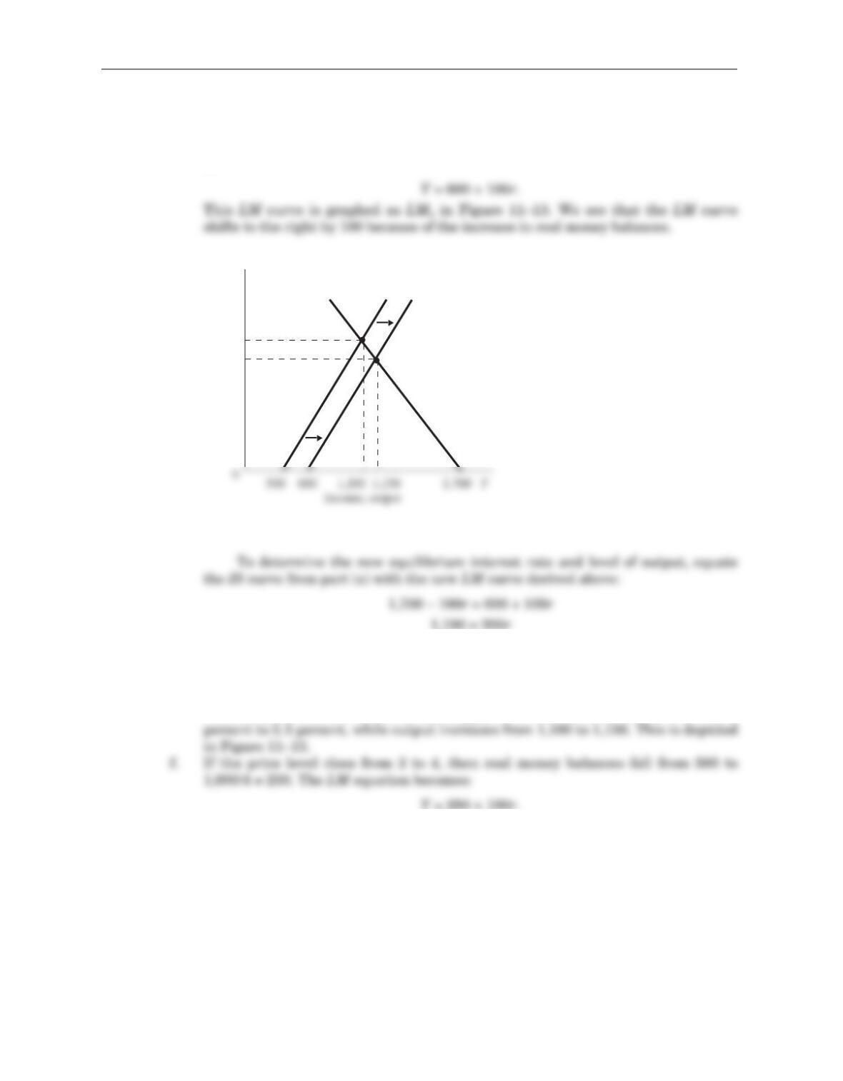
d. If government purchases increase from 100 to 150, then the IS equation becomes:
Y= 200 + 0.75(Y– 100) + 200 – 25r+ 150.
Simplifying, we find:
Y= 1,900 – 100r.
This IS curve is graphed as IS2in Figure 11–12. We see that the IS curve shifts to
the right by 200.
By equating the new IS curve with the LM curve derived in part (b), we can
solve for the new equilibrium interest rate:
1,900 – 100r= 500 + 100r
1,400 = 200r
7 = r.
104 Answers to Textbook Questions and Problems
LM
r
IS2
IS1
8
Figure 11–12
e. If the money supply increases from 1,000 to 1,200, then the LM equation becomes:
(1,200/2) = Y– 100r,
or
5.5 = r.
Substituting this into either the IS or the LM equation, we find
Y= 1,150.
Therefore, the increase in the money supply causes the interest rate to fall from 6
Chapter 11 Aggregate Demand II 105
IS
r
6.0
5.5
Interest rate
100
LM1LM2
Figure 11–13
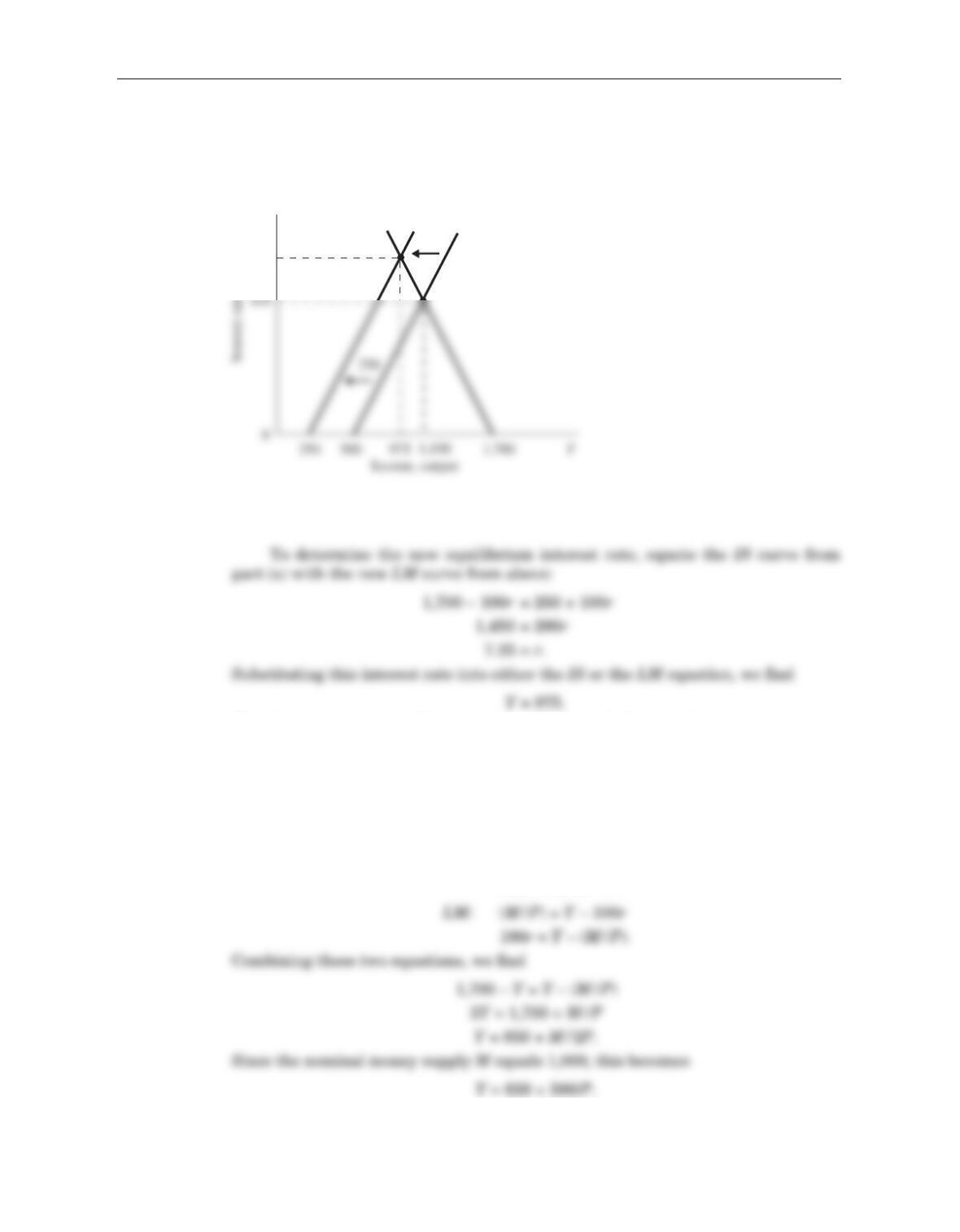
As shown in Figure 11–14, the LM curve shifts to the left by 250 because the
increase in the price level reduces real money balances.
Therefore, the new equilibrium interest rate is 7.25, and the new equilibrium
level of output is 975, as depicted in Figure 11–14.
g. The aggregate demand curve is a relationship between the price level and the
level of income. To derive the aggregate demand curve, we want to solve the IS
and the LM equations for Yas a function of P. That is, we want to substitute out
for the interest rate. We can do this by solving the IS and the LM equations for
the interest rate:
IS: Y= 1,700 – 100r
100r= 1,700 – Y.
106 Answers to Textbook Questions and Problems
IS
r
7.25
LM2LM1
Figure 11–14
Chapter 11 Aggregate Demand II 107
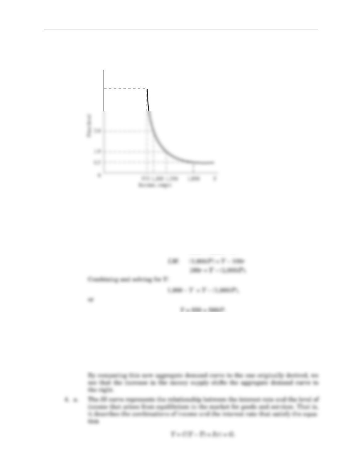
This aggregate demand equation is graphed in Figure 11–15.
How does the increase in fiscal policy of part (d) affect the aggregate demand
curve? We can see this by deriving the aggregate demand curve using the IS equa-
tion from part (d) and the LM curve from part (b):
IS: Y= 1,900 – 100r
100r= 1,900 – Y.
By comparing this new aggregate demand equation to the one previously derived,
we can see that the increase in government purchases by 50 shifts the aggregate
demand curve to the right by 100.
How does the increase in the money supply of part (e) affect the aggregate
demand curve? Because the AD curve is Y= 850 + M/2P, the increase in the
money supply from 1,000 to 1,200 causes it to become
Y= 850 + 600/P.
P
4.0
Figure 11–15