hold.
Changes in the nominal exchange rate reflect:
2 Exchange Rates in the Short Run: Deviations from Uncovered Interest
Parity
The UIP condition relies on arbitrage to ensure that the expected return on foreign
deposits equals the return on domestic deposits in the same currency terms. There is still
APPLICATION
The Carry Trade
UIP: Home interest rates should equal the foreign interest rate plus the expected rate of
depreciation in the home currency. If UIP holds, an investor cannot earn riskless profit
The Long and Short of It In practice, investors do engage in carry trade and earn large
profits from doing so. Investors borrow in low-interest currencies (“go short”) and invest
in higher-interest currencies (“go long”).
Figure 22-4, panel (a), reports profits from carry trade involving borrowing in the
low-interest Japanese yen money market and investing in high-interest Australian dollar
money market accounts for one month. During 2001, we observe a steady increase in the
Using some language from financial markets, we can consider the role of leverage
and margin. Suppose that you have $2,000 to invest and borrow an additional $48,000 in
yen from a bank in Japan. You now have 25 times your own $2,000 capital, a leverage
ratio of 25. You conduct carry trade, investing $50,000 in the Australian dollar. If you
Carry Trade Summary We observe the following from carry trade data:
■ Even if expected returns from arbitrage are equal to zero, actual profits are often
H E A D L I N E S
Mrs. Watanabe’s Hedge Fund
This article summarizes the 2006–2007 experiences of individual Japanese investors with
carry trade.
Background:
Total profits from carry trade involving the yen totaled $4 trillion in 2006, according to
an OECD estimate.
■ Middle-class Japanese homemakers, “Mrs. Watanabes,” have engaged in currency
speculation, attempting to earn profits from carry trade in lieu of investing in low–
Key statistics:
■ Japanese homemakers are largely responsible for managing the nation’s $12.5
trillion in household savings.
■ A small fraction of these savings is invested in currency speculation, margin
Lessons:
■ Carry trade involves considerable risk.
Discussion questions:
■ Consider the data reported in Figure 22-4. Do you expect that margin trading
involving borrowing in yen and investing in Australian dollars will be profitable
in the long term? Why might currency traders engage in these activities in the
immediate term?
APPLICATION
Peso Problems
It’s possible to earn positive returns trading currencies that are pegged. For example, both
Hong Kong’s dollar and many countries in the Middle East and the Caribbean are pegged
to the U.S. dollar. Argentina’s peso was pegged to the U.S. dollar until the financial crisis
Hong Kong:
■ Panel (a) shows the interest rate differential between Hong Kong and the U.S. was
near zero most of the time. Hong Kong’s peg was considered the most solid in the
world.
■ This is not surprising. Hong Kong maintains a currency board with large foreign
currency reserves.
Argentina:
■ In 2001, an economic and banking crisis led to worries of default, driving down
the value of the Argentine peso.
The peso problem refers to the currency premiums associated with a pegged currency.
The collapse of a peg can be viewed as infrequent, and even unlikely, as in the case of
Hong Kong. However, Argentina’s experience shows us that investors can suffer
The Efficient Markets Hypothesis
This section develops a familiar model from financial economics: the efficient markets
hypothesis. The model is used to examine whether carry trade profits disprove UIP.
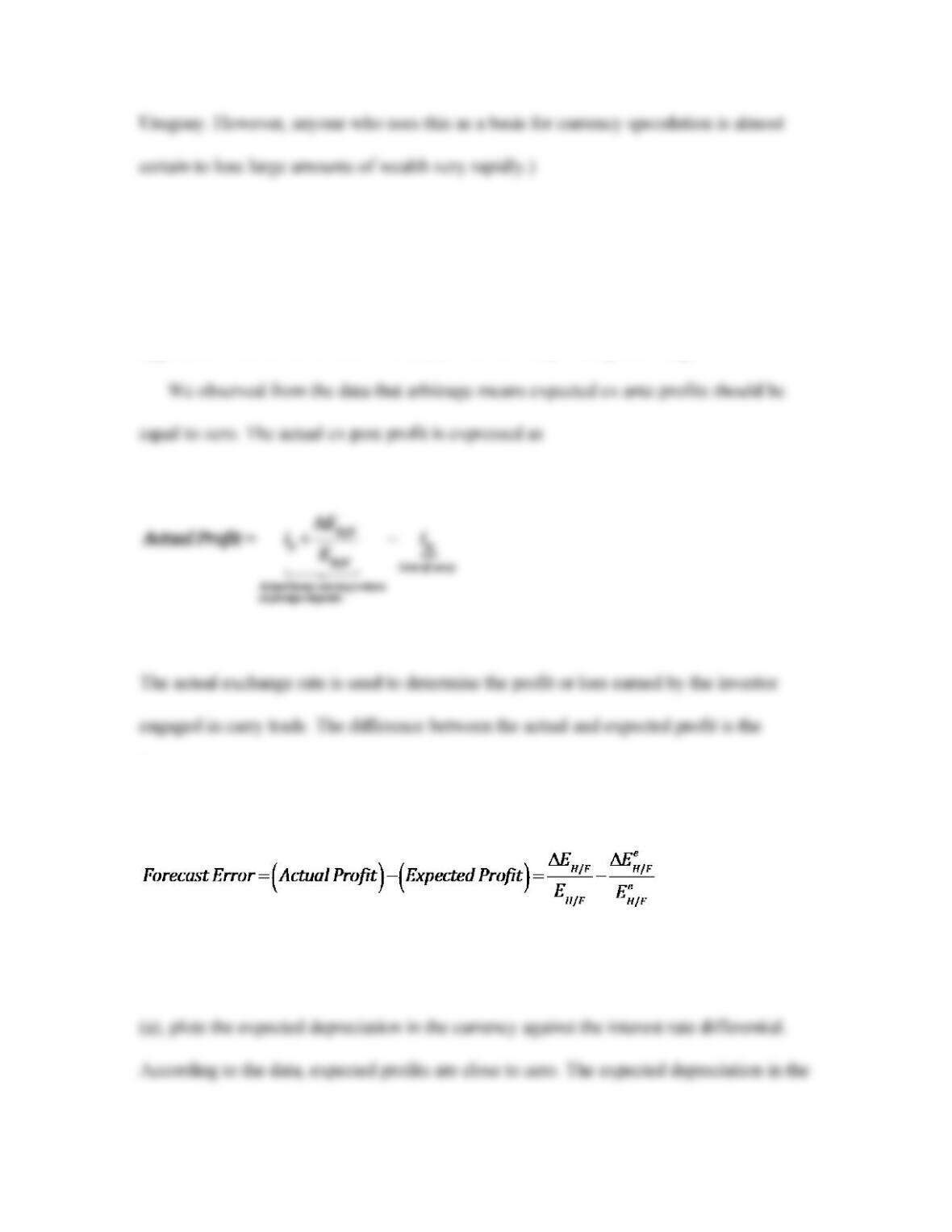
forecast error:
Expected Profits The UIP condition has to do with ex ante profits. Figure 22-6, panel
Actual Profits Figure 22-6, panel (b), reports the actual depreciation against the interest
rate differential. From this figure, we see that actual profits are made and that the data are
The UIP Puzzle By itself, the fact that profits are positive does not imply UIP is
incorrect. If the distribution of profits is random, UIP would hold on an expected value
basis. Unfortunately, the deviations are systematic. If these actual profits can be
forecasted, this would violate a tenet of finance theory. The rational expectations
hypothesis says that forecast errors should be random or unpredictable. That is, investors
do not make systematic mistakes.
A related theory, the efficient markets hypothesis, says that financial markets are
An empirical test of UIP combined with the rational expectations and efficient
markets hypothesis fails, suggesting the forex market is an inefficient market. This
Limits to Arbitrage
The explanations for the existence of predictable profits are based on limits to arbitrage.
Trade Costs Are Small It’s tempting to simply list the same frictions we saw earlier in
this chapter: trade costs, nontraded goods, and the speed of convergence to equilibrium.
Unfortunately, that approach will not work here. Trade costs in financial transactions are
trivially small. While there are bid–ask spreads in currency trading markets (and most
other financial markets), the size of the spread is not large enough to explain the profits
we saw earlier.
Risk Versus Reward We can look at the relationship between the profits earned on carry
trade and compare these returns with the risks to which investors are exposed. Using the
data reported in Figure 22-6, panel (b), we observe that a positive 1% interest differential
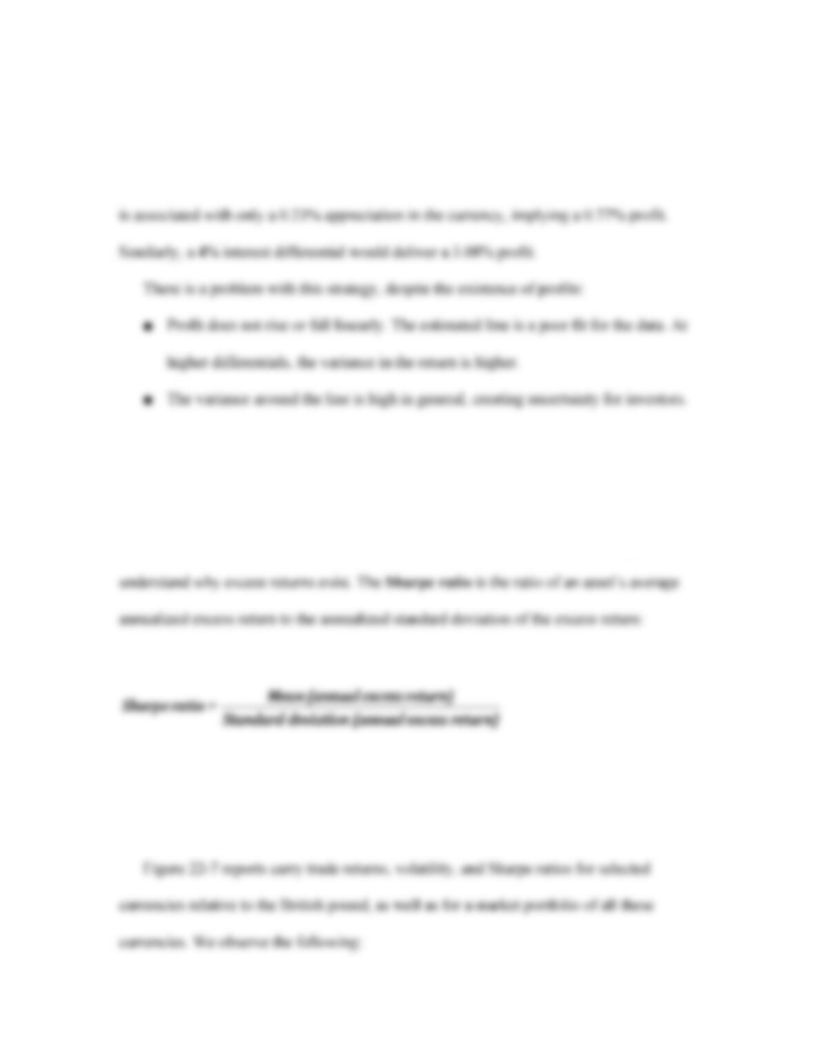
The Sharpe Ratio and Puzzles in Finance Carry trade profits are the difference
between risky foreign rates of return and safer domestic returns. An excess return is
earned on that difference. We can use one of the standard tools of finance to help us
A higher ratio indicates that an asset with a given level of risk earns a higher return. A
lower ratio suggests the asset has a low return relative to the degree of risk.
■ Returns are positive for all these currencies; equal to roughly 4% per year.
■ The standard deviation of these returns is very high, with an average of 6%.
■ The Sharpe ratio is 0.6 for the diversified portfolio. The average of the individual
Predictability and Nonlinearity We have already seen that trade costs are too small and
that the risk‒reward trade-off cannot explain the existence of predictable profits in the
forex market. Perhaps the linear model is a poor description of the forex market.
Nonlinear models reveal that low–interest differentials are associated with very low
Conclusion
The data show there are predictable, positive returns in the forex market. By itself, this is
not a violation of UIP. When we add efficient markets, the existence of such profits
3 Debt and Default
This section examines the role of sovereign default in international capital markets.
Sovereign default occurs when a sovereign government fails to meet its obligations to
make payments on debt held by foreigners.
Sovereign defaults have a very long history:
■ Greek municipalities defaulted on loans from the Delos Temple in the fourth
■ The U.S. federal government has avoided default during its short history, although
Today’s advanced economies do not default, but it is a recurring problem in emerging
markets and developing countries:
■ Argentina, Brazil, Mexico, Turkey, and Venezuela have defaulted five to nine
Puzzle: Why do emerging markets and developing countries get into default trouble at
lower levels of debt relative to advanced economies?
■ As of late 2010, a number of European countries have gone to the brink of
A Few Peculiar Facts About Sovereign Debt
Debtors are almost never forced to pay. There is virtually no way to force a sovereign
government to honor its debt obligations. Repayment of debt is largely a choice for the
borrowing government. How painful does repayment have to get before default occurs?
■ Financial market penalties:
● Debtors that default are excluded from credit markets for some period after
■ Broader macroeconomic costs:
● Lost investment, lost trade, or lost output caused by adverse financial market
Summary Sovereign debt is a contingent claim: governments will repay only if the
A Model of Default, Part One: The Probability of Default
Assumptions In the model, a country will borrow to smooth its consumption. Repayment
of the debt is contingent on losses associated with output fluctuations.
■ Fluctuations in output are exogenous, with output, Y, taking on some value
between a minimum, − V, and a maximum, . The variable V is therefore a
measure of output volatility.
The Borrower Chooses Default Versus Repayment Assume the borrower suffers some
cost associated with defaulting, cY, leaving (1 − c)Y available for consumption. The
choice facing the government is whether to default or repay the loan.
■ If the government repays the loan, output available for consumption will be Y − (1
+ rL)L.
■ RR is the repayment line, with a slope of 1. Each extra dollar in output goes
toward consumption, net of debt repayment.
■ NN is the nonrepayment line, with a slope of (1 − c). Each extra dollar of output
results in only (1 − c) dollars of consumption.
An Increase in the Debt Burden Suppose there is an exogenous increase in the debt
burden. (This could be caused by an increase in the lending rate, an increase in the
volume of borrowing, or some combination of the two.) The new burden is (1 + r
′
L)L
′
.
This scenario is shown in Figure 22-9.
■ The RR line shifts down to R
′
R
′
.
An Increase in Volatility of Output Suppose the potential decrease in output is larger,
so V increases to V
′
. This case is illustrated in Figure 22-10.
■ Consumption levels along RR and NN are unaffected.
■ There is the potential for greater losses in output, making default more likely.
The Lender Chooses the Lending Rate Based on the probability of repayment, we can
determine the interest rate the lender will charge for a loan. Competition in financial
markets means that lenders simply will break even, so the lender will set the interest rate
such that the revenues exactly equal the costs. The break-even condition follows:
The term on the left-hand side of the expression is the revenue the lender expects to
collect. The term on the right-hand side is the cost of forgone investment opportunities in
financial markets.
APPLICATION
Is There Profit in Lending to Developing Countries?
The empirical evidence suggests that lenders do not make large profits on loans to debtor
countries. This application considers a study of returns on government debt in 22
borrower countries from 1970 to 2000 (Klingen, Weder, & Zettlemeyer, 2004). Figure
22-20 reports the results of this analysis of ex post returns.
■ Average returns = 9.1% per year:
● 8.6% return on 3-year U.S. government bonds
● 9.2% return on 10-year U.S. government bonds
A Model of Default, Part Two: Loan Supply and Demand
This model will be useful in analyzing the equilibrium behavior of loans, the interest rate
charged on these loans, and the probability of repayment.
Loan Supply Suppose that output volatility, V, is low. The probability of repayment is
shown in Figure 22-12, panel (a). Loan supply, LS(V), is illustrated in panel (b), as a
function of the lending rate (= risk–free rate + risk premium).
■ When the loan amount is low, less than some value LV:
● the loan will be repaid with 100% probability.
● the lending rate has no risk premium, so rL = r.
● the loan supply curve has a zero slope at r.
■ As the loan amount increases, above LV (but below LMAX):
● the probability of loan repayment decreases.
● the lending rate increases with the risk premium, so rL > r.
Loan Demand The slope of LD(V) depends on two factors: the lending rate, rL, and
output volatility, V. Figure 22-21, panel (b), illustrates loan demand as a decreasing
function of the lending rate, rL.
An Increase in Volatility Figure 22-22 illustrates how an increase in output volatility
affects loan demand.
■ Panel (a):
● An increase in V leads to an increase in the probability of default. As V rises,
the probability of repayment drops below 100% at a lower level of debt.
■ Panel (b):
● Loan supply decreases: For a given loan amount, L (above L
′
V and below
LMAX), the equilibrium lending rate is higher because: