Economics Chapter 11 France And Germany Respectively This Was Matched

Chapter 11

Aggregate Supply and the Phillips Curve

◼ Chapter Outline, Overview, and Teaching Tips

Chapter Outline

The Phillips Curve

Phillips Curve Analysis in the 1960s

Policy and Practice: The Phillips Curve Tradeoff and Macroeconomic Policy in the 1960s

The Friedman-Phelps Phillips Curve Analysis

The Modern Phillips Curve with Adaptive (Backward-Looking) Expectations

The Aggregate Supply Curve

Long-Run Aggregate Supply Curve

Short-Run Aggregate Supply Curve

Shifts in Aggregate Supply Curves

Shifts in the Long-Run Aggregate Supply Curve

Chapter Overview and Teaching Tips

The last building block of the AD/AS framework is the aggregate supply curve. This chapter develops the

aggregate supply curve from Phillips curve analysis. To give students the intuition behind the Phillips

curve, the chapter starts by showing how Phillips curve analysis has evolved through time. The Policy and

110 Mishkin • Macroeconomics: Policy and Practice, Second Edition

◼ Answers to End of Chapter Review Questions and Problems

Answers to Review Questions

The Phillips Curve

1. The short-run Phillips curve describes a negative relationship between unemployment and inflation.

2. According to the long-run Phillips curve, unemployment moves to a natural rate regardless of the rate

of inflation, so there is no long-run tradeoff between inflation and unemployment that policy makers

3. According to the expectations-augmented Phillips curve, the inflation rate depends on expected

inflation and the unemployment gap, which measures tightness in labor markets as the difference

4. Adaptive expectations are formed by looking at past values of the variable being forecast. (Because

they look at the past, adaptive expectations sometimes are called backward-looking expectations.)

5. In modern Phillips curve analysis, the rate of inflation increases one-for-one with changes in expected

inflation and price shocks and moves inversely to the unemployment gap. Price shocks and changes

The Aggregate Supply Curve

6. The aggregate supply curve shows the relationship between the total quantity of output supplied and

the inflation rate. In the long run, the amount of output an economy can produce is determined by its

7. Okun’s Law relates the unemployment gap U − Un, where U is the unemployment rate and Un is the

natural rate of unemployment, to the output gap Y − YP, where Y is aggregate output and YP is the

economy’s potential output. The relationship between the two gaps is negative because when the

Chapter 11 Aggregate Supply and the Phillips Curve 111

8. When output increases relative to potential output, Y − YP increases. At the same time, according to

Okun’s Law, the unemployment rate is falling relative to the natural rate of unemployment, which

Shifts in Aggregate Supply Curves

9. Shifts in the long-run aggregate supply curve result from changes in the total quantities of capital and

10. The short-run aggregate supply curve shifts upward when expected inflation increases, when positive

Answers to Problems

The Phillips Curve

1.

112 Mishkin • Macroeconomics: Policy and Practice, Second Edition

2.

3. a. Substituting the values of expected inflation and the natural rate of unemployment yields the

following expression:

3 0.5( 5)U



= − −

. According to this expression, inflation rates are 3.5

percent, 3 percent, and 2.5 percent when unemployment rates are 4 percent, 5 percent, and 6

Chapter 11 Aggregate Supply and the Phillips Curve 113

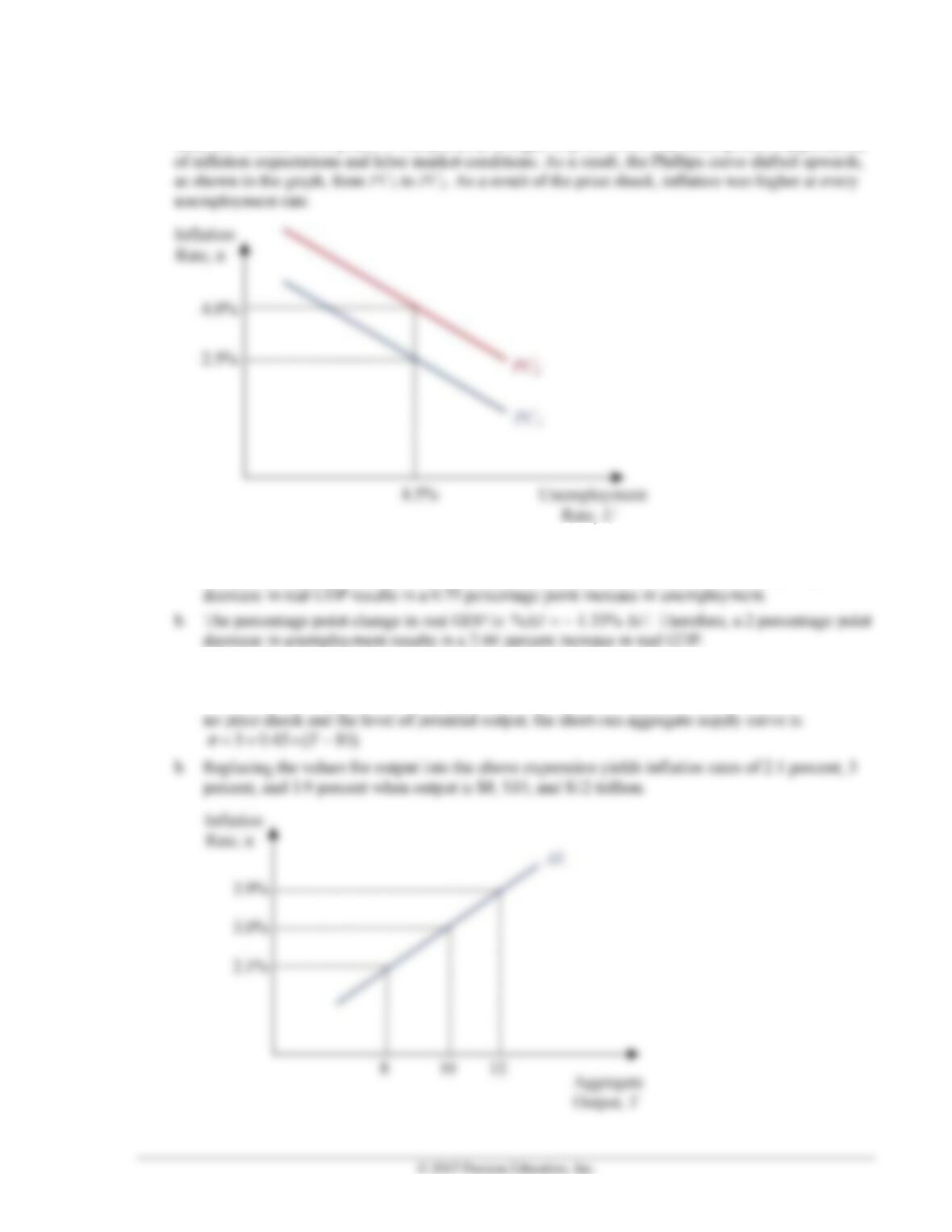
4. The modern Phillips curve allows for shifts in the Phillips curve that arise from price shocks. In this

case, the increase in oil prices is interpreted as a negative price shock that raises prices independently

The Aggregate Supply Curve

5. a. The percentage point change in unemployment is: % = − 0.75  (%Y). Therefore, a 1 percent

6. a. First substitute the unemployment gap with Okun’s Law into the Phillips curve to get:

0.6 ( 0.75 ( )) .

eP

YY

  

= −  −  − +

According to the assumptions about inflation expectations,

114 Mishkin • Macroeconomics: Policy and Practice, Second Edition

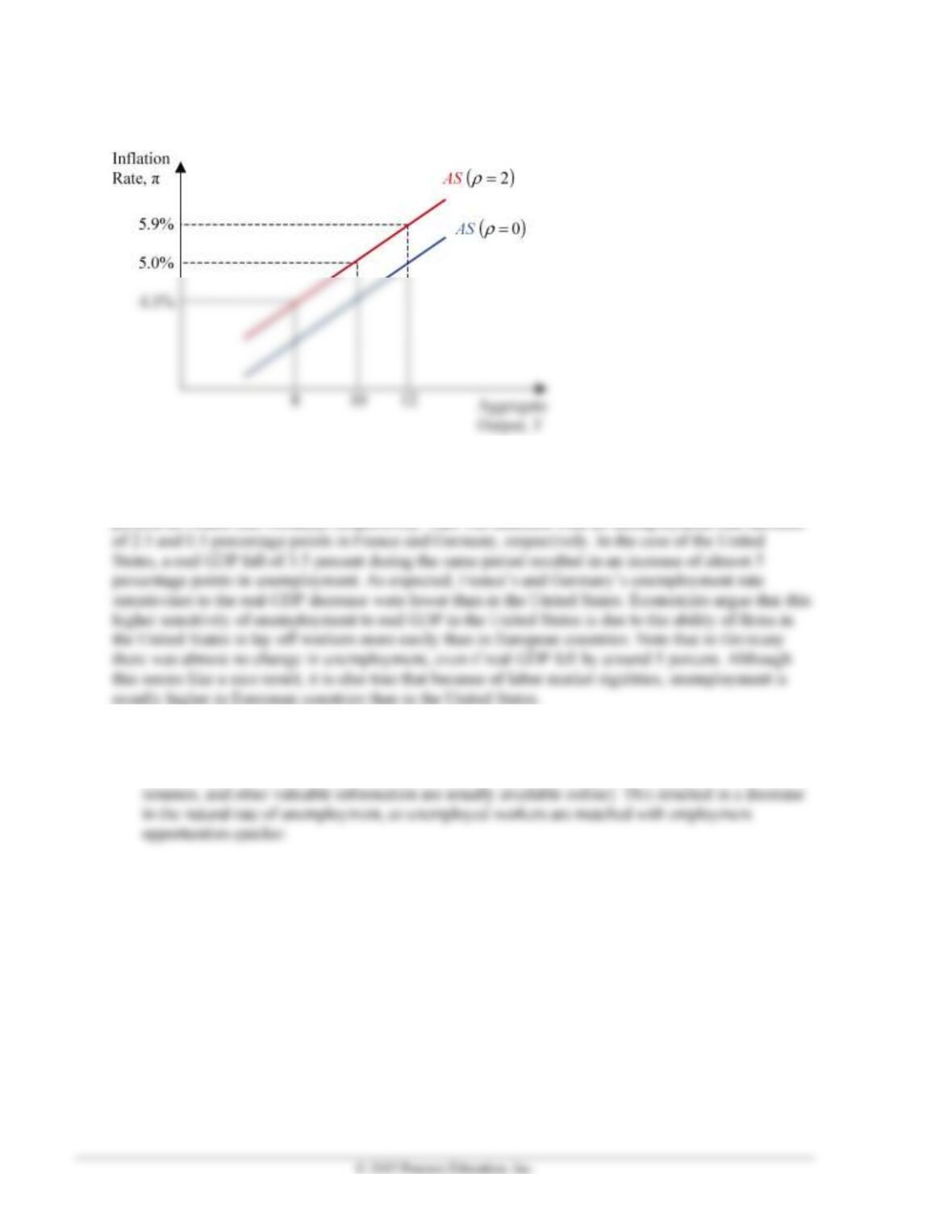
7. The new short-run aggregate supply curve is:

3 0.45 ( 10) .Y



= +  − +

8. Okun’s Law held for these three countries. In all cases, a decrease in real GDP was matched with an

increase in unemployment. However, more rigid labor markets in Germany and France prevented a

higher response in unemployment. During 2008–2009, real GDP decreased by 2.5 percent and 5

percent in France and Germany, respectively. This was matched with an unemployment rate increase

Shifts in Aggregate Supply Curves

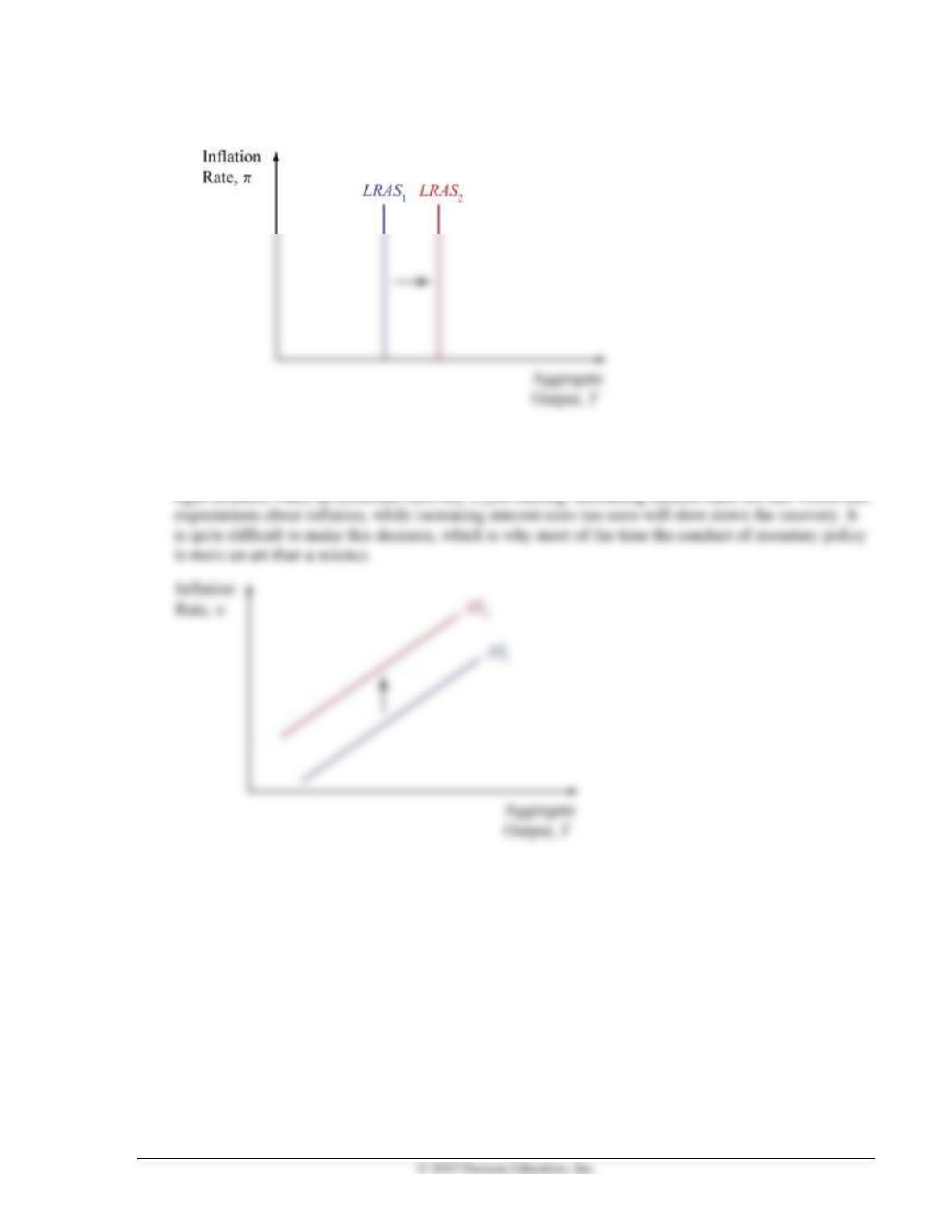
9. a. The Internet reduced the amount of time and money spent looking for a job. It also allowed for an

increased flow of information between potential employees and employers (e.g., job descriptions,

Chapter 11 Aggregate Supply and the Phillips Curve 115

b. Graphically, the long run aggregate supply curve shifts to the right:

10. If the public assumes that the current Fed officials are not that worried about inflation, expected inflation

will increase, shifting the short-run aggregate supply curve upward and to the left. There are periods

when Fed officials are in the difficult position of having to choose when to increase interest rates to

116 Mishkin • Macroeconomics: Policy and Practice, Second Edition

◼ Answers to Data Analysis Problems

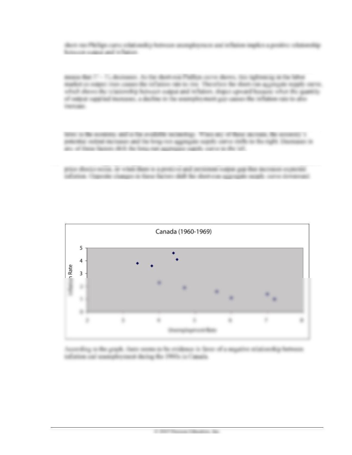
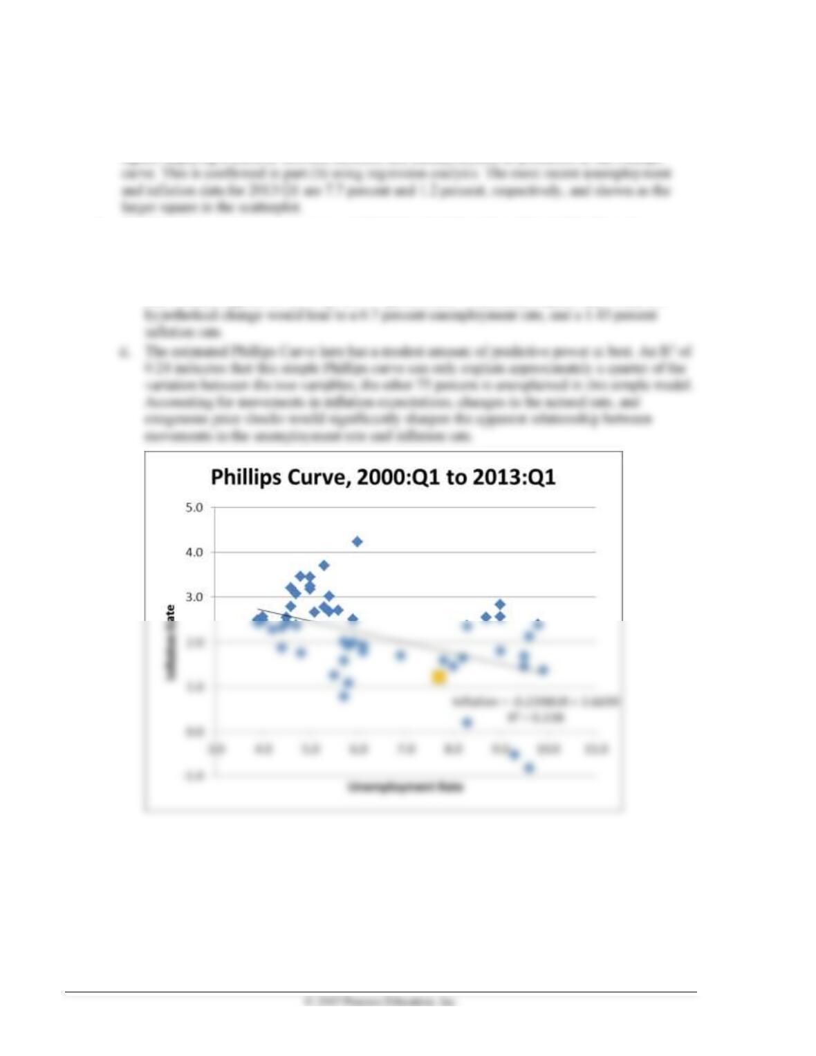
1. a. See figure below. The scatterplot does seem to have a downward slope on inspection of the

figure, implying a tradeoff between inflation and unemployment as predicted by the Phillips

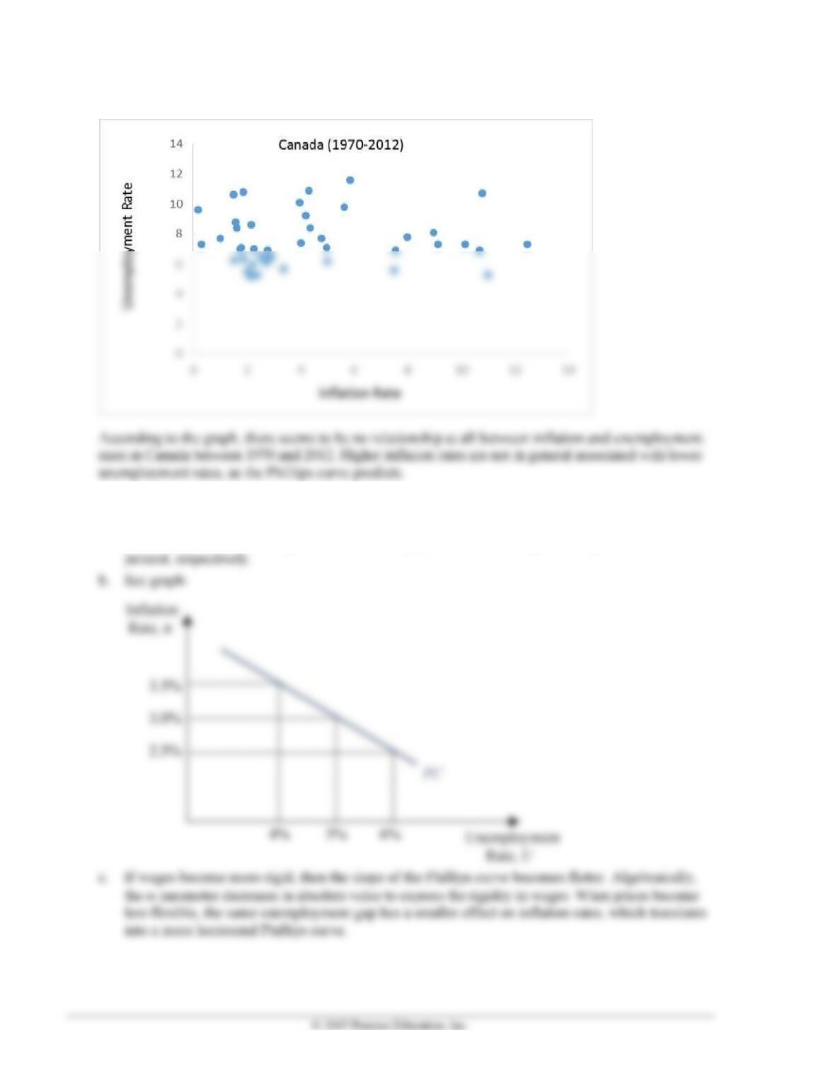
b. The fitted line equation is Inflation = –0.2398UR + 3.6699, with an R² = 0.238. Thus, the

negative slope of the fitted line indicates a tradeoff between inflation and unemployment.

i. According to the fitted regression, a decrease in unemployment of 1 percentage point would

lead to an increase in inflation of 0.23 percentage points. The most current unemployment

and inflation figures for 2013:Q1 are 7.7 percent and 1.2 percent, respectively. Thus, this

Chapter 11 Aggregate Supply and the Phillips Curve 117

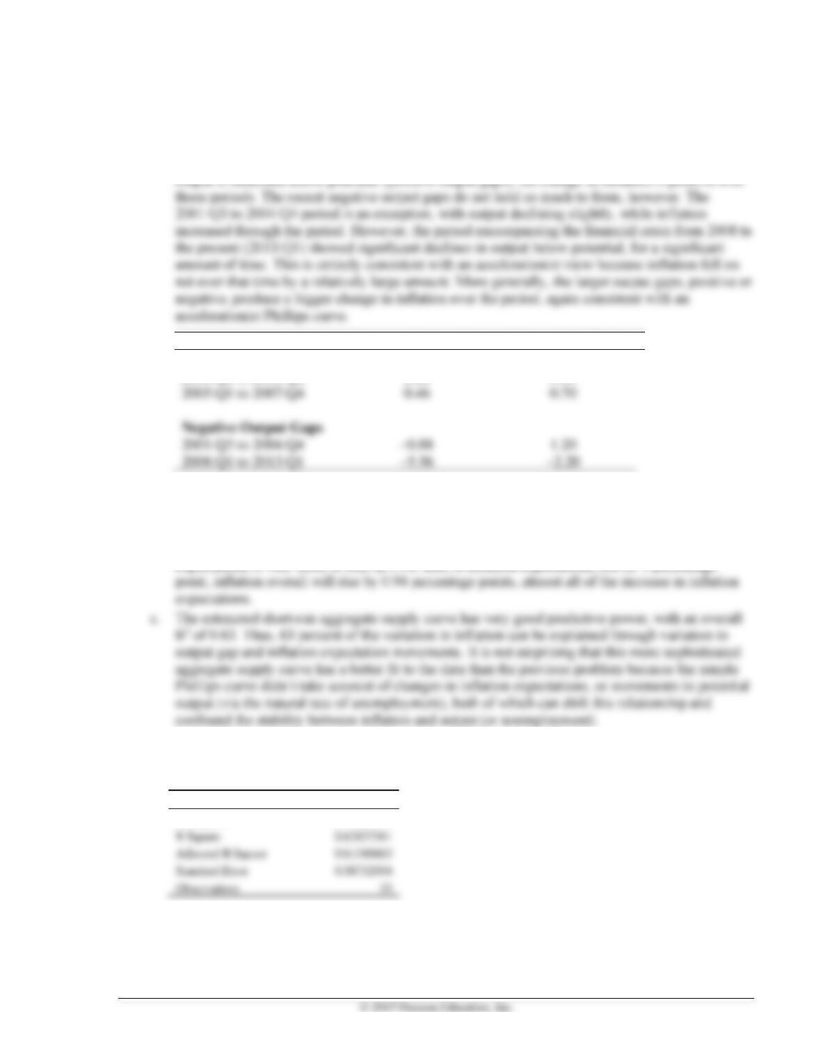
2. a. Positive output gaps: 2000:Q1 to 2001:Q2; 2005:Q1 to 2007:Q4. Negative output gaps: 2001:Q3

to 2004:Q4; 2008:Q1 to 2013:Q1

b. See table below.

c. For the most part, the table does fit the view of an accelerationist Phillips curve. In periods when

Average Output Gap

Change in Inflation

Positive Output Gaps

2000:Q1 to 2001:Q2

2.22

0.80

2005:Q1 to 2007:Q4

0.46

0.70

Negative Output Gaps

2001:Q3 to 2004:Q4

1.20

2008:Q1 to 2013:Q1

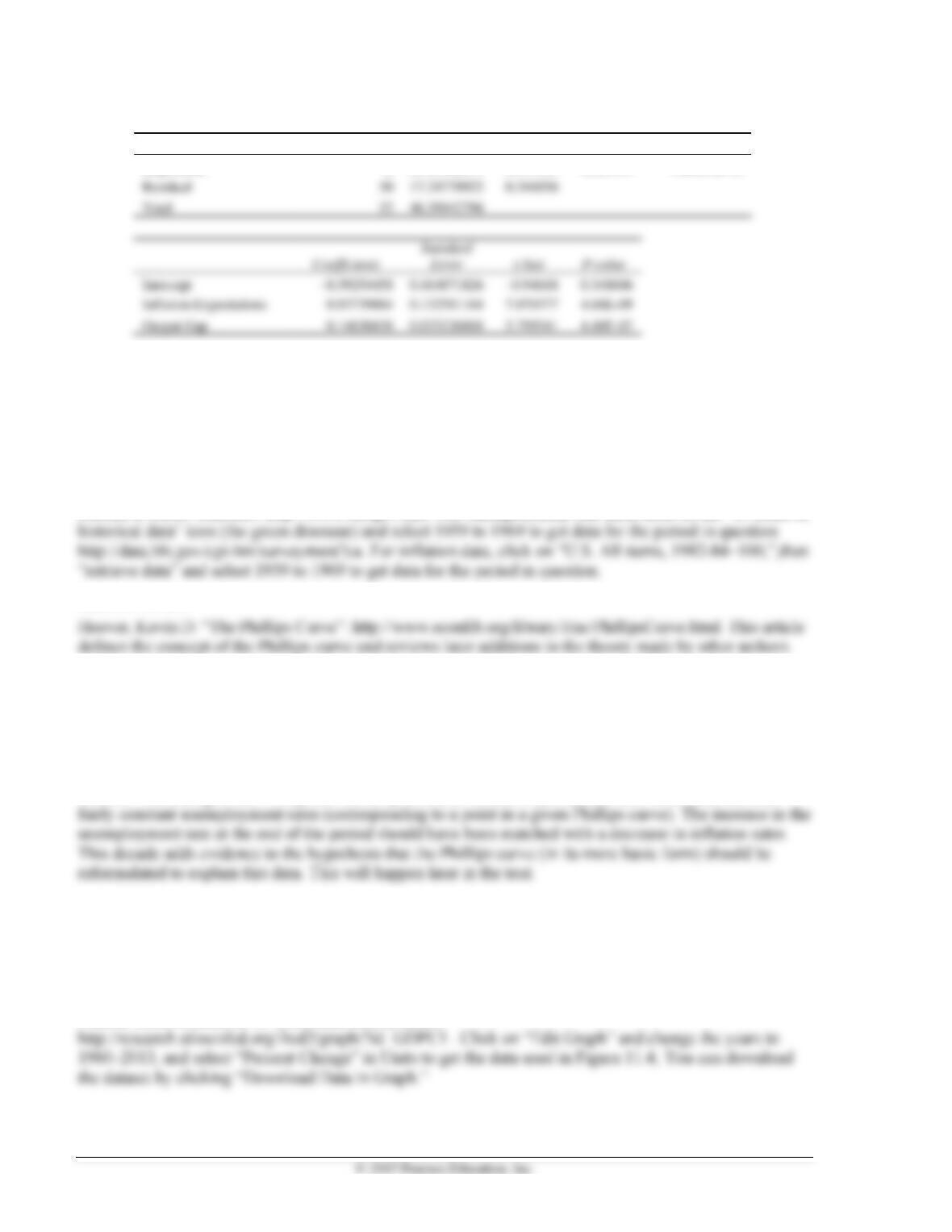
3. a. See regression output below, for 2000:Q1 to 2013:Q1.

b. The results are entirely consistent with a short-run aggregate supply curve: The slope of the curve

is positive, with an estimated (γ) coefficient of 0.15 meaning if the output gap rises by 1

percentage point, inflation will rise by 0.15 percentage points. The coefficient on inflation

expectations is very close to one, at 0.94; thus, if inflation expectations rise by 1 percentage

d. In 2013:Q1, the output gap was –5.8 percent; thus, if policy makers were to close this output gap,

the short-run aggregate supply curve would predict a 0.15 × (5.8%) = 0.87 percentage point

increase in inflation as a result.

Regression Statistics

Multiple R

0.79263838

R Square

0.62827561

Standard Error

0.58732954

Observations

118 Mishkin • Macroeconomics: Policy and Practice, Second Edition

ANOVA

df

SS

MS

F

Significance F

Regression

2

29.15162874

14.57581

42.25413

1.80105E-11

Inflation Expectations

0.132581164

7.070377

◼ Data Sources, Related Articles, and Discussion Questions

A. For Information About Policy and Practice: The Phillips Curve Tradeoff and

Macroeconomic Policy in the 1960s

Data Sources

Bureau of Labor Statistics: http://www.bls.gov/cps/. For unemployment rate data, click on the “10 years of

During the 2000–2010 period, inflation rates in the United States fluctuated around a fairly low average of

2.5 percent annual rate, while the unemployment rate increased sharply at the end of the period (from around

5 percent in the early 2000s to almost 10 percent in 2009). Would this data be consistent with the Philips

curve concept?

Answer: According to the Phillips curve, fairly constant inflation rates should have been matched with

B. For Information About Okun’s Law

Data Sources

Bureau of Labor Statistics: http://www.bls.gov/cps/. For unemployment rate data, click on the “10 years of

historical data” icon (the green dinosaur) and select 1960 to 2013 to get data used for Figure 11.4.

Federal Reserve Bank of St. Louis data base (FRED):

Chapter 11 Aggregate Supply and the Phillips Curve 119

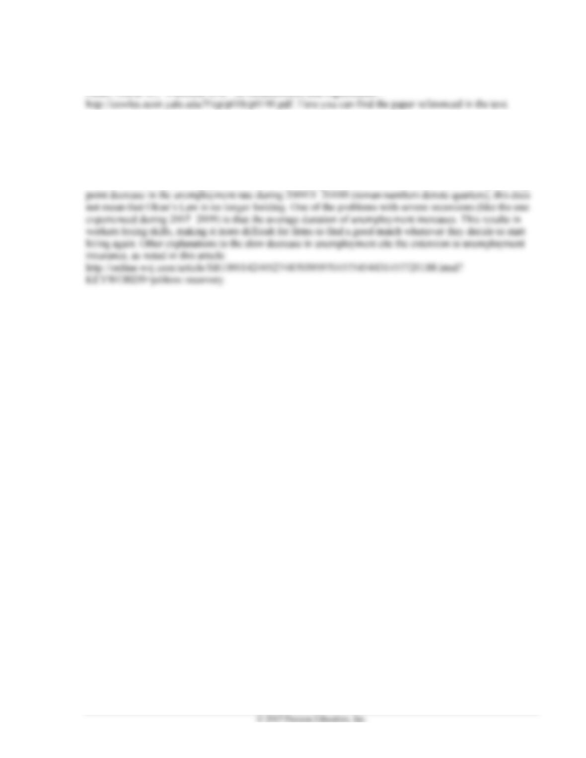
Discussion Question

During the second semester of 2009 and the first semester of 2010, the GDP growth rate became positive.

However, percentage changes in the GDP growth rate were not matched by half percentage point decreases

in the unemployment rate during that period. Would this suggest that Okun’s Law is no longer valid?

Answer: Even if a percentage point increase in the GDP growth rate was not matched with half a percentage