interactive activity
Chapter 11
Behind the Supply
Curve: Inputs and Costs
1. Changes in the prices of key commodities have a significant impact on a compa-
ny’s bottom line. For virtually all companies, the price of energy is a substantial
portion of their costs. In addition, many industries—such as those that produce
beef, chicken, high-fructose corn syrup and ethanol—are highly dependent on
the price of corn. In particular, corn has seen a significant increase in price.
a. Explain how the cost of energy can be both a fixed cost and a variable cost for
a company.
b. Suppose energy is a fixed cost and energy prices rise. What happens to the
company’s average total cost curve? What happens to its marginal cost curve?
Illustrate your answer with a diagram.
c. Explain why the cost of corn is a variable cost but not a fixed cost for an etha-
nol producer.
d. When the cost of corn goes up, what happens to the average total cost curve of
an ethanol producer? What happens to its marginal cost curve? Illustrate your
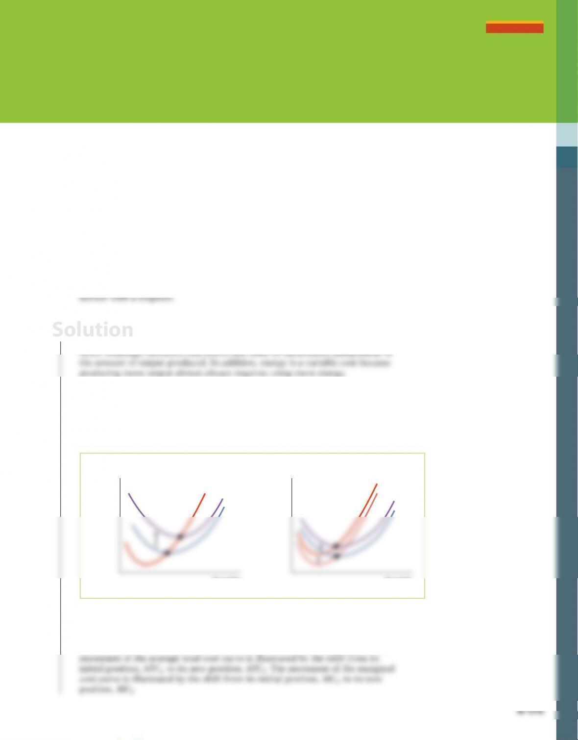
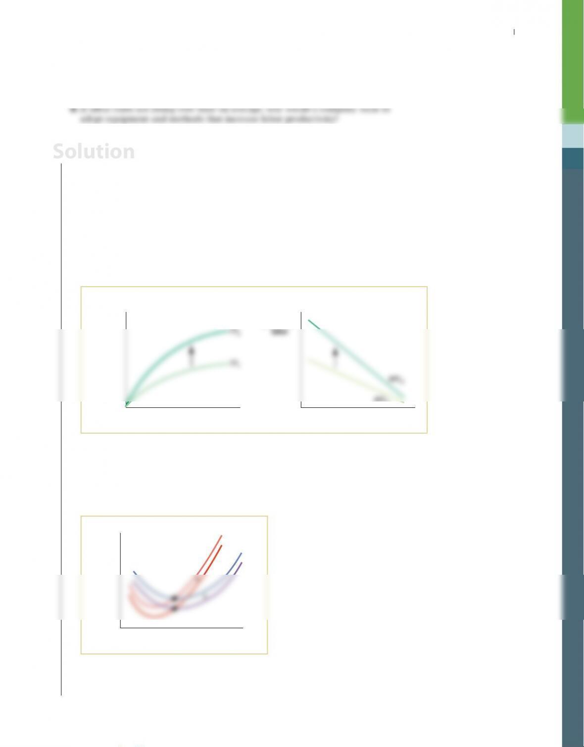
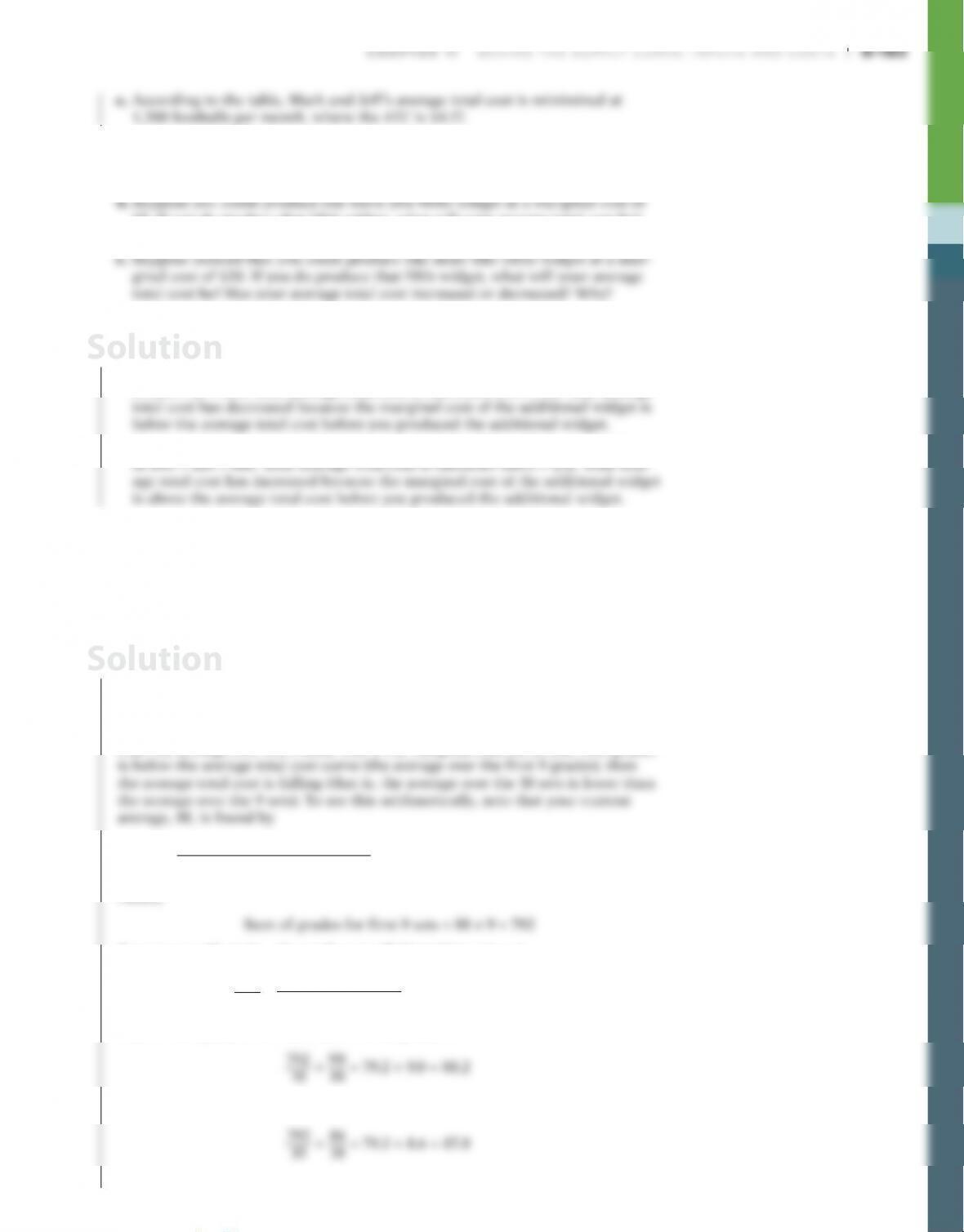
1. a. Energy required to keep a company operating regardless of how much out–
put is produced represents a fixed cost, such as the energy costs of operating
b. When fixed costs increase, so will average total costs. The average total
cost curve will shift upward. In panel (a) of the accompanying diagram,
this is illustrated by the movement of the average total cost curve from its
initial position, ATC1, to its new position, ATC2. The marginal cost curve is
not affected if the variable costs do not change. So the marginal cost curve
remains at its initial position, MC.
Cost
of
unit
Cost
of unit
Quantity Quantity
MC
MC2
MC1
ATC2ATC2
ATC1
ATC1
(b) A Rise in the Price of Corn(a) A Rise in the Price of Energy
c. Since corn is an input into the production of ethanol, producing a larger quan-
tity of ethanol requires a larger quantity of corn, making corn a variable cost.
d. When variable costs increase, so do average total costs and marginal costs.
Both curves will shift upward. In panel (b) of the accompanying diagram, the
Solution
S-176 Chapter 11 Behind the Supply Curve: inputS and CoStS
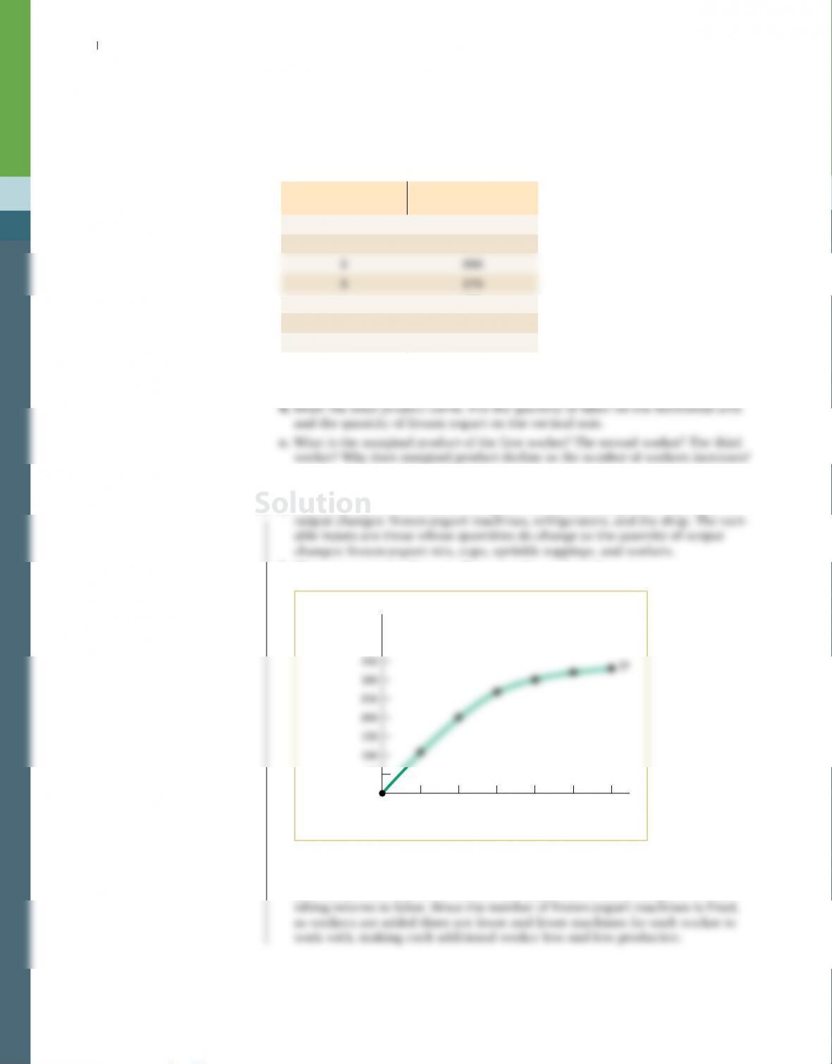
2. Marty’s Frozen Yogurt is a small shop that sells cups of frozen yogurt in a uni-
versity town. Marty owns three frozen-yogurt machines. His other inputs are
refrigerators, frozen-yogurt mix, cups, sprinkle toppings, and, of course, work-
ers. He estimates that his daily production function when he varies the number
of workers employed (and at the same time, of course, yogurt mix, cups, and so
on) is as shown in the accompanying table.
Quantity of labor
(workers)
Quantity of frozen
yogurt (cups)
0 0
1110
4300
5320
6330
a. What are the fixed inputs and variable inputs in the production of cups of fro–
zen yogurt?
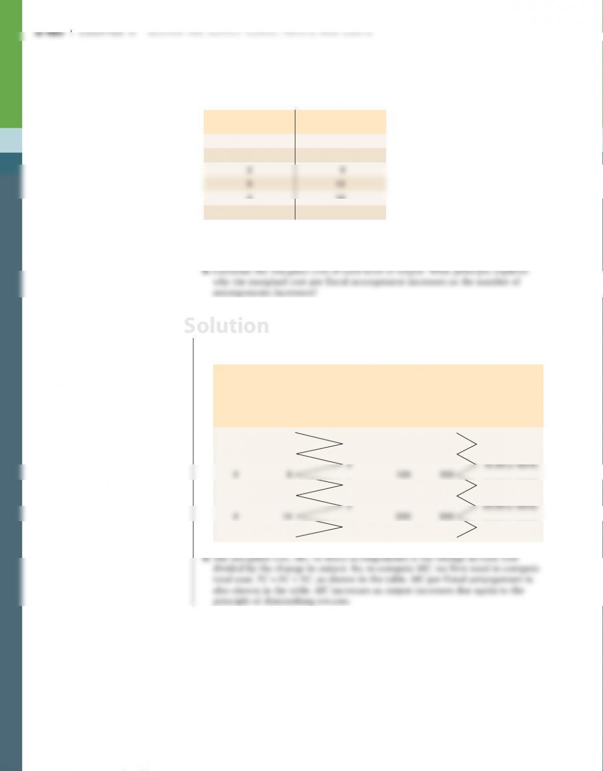
2. a. The fixed inputs are those whose quantities do not change as the quantity of
b. The accompanying diagram illustrates the total product curve.
56
43210
50
Quantity of
fr
ozen yogurt
(cups)
Quantity of labor (workers)
c. The marginal product, MPL, of the first worker is 110 cups. The MPL of the
second worker is 90 cups. The MPL of the third worker is 70 cups. The MPL
declines as more and more workers are added due to the principle of dimin-
Solution
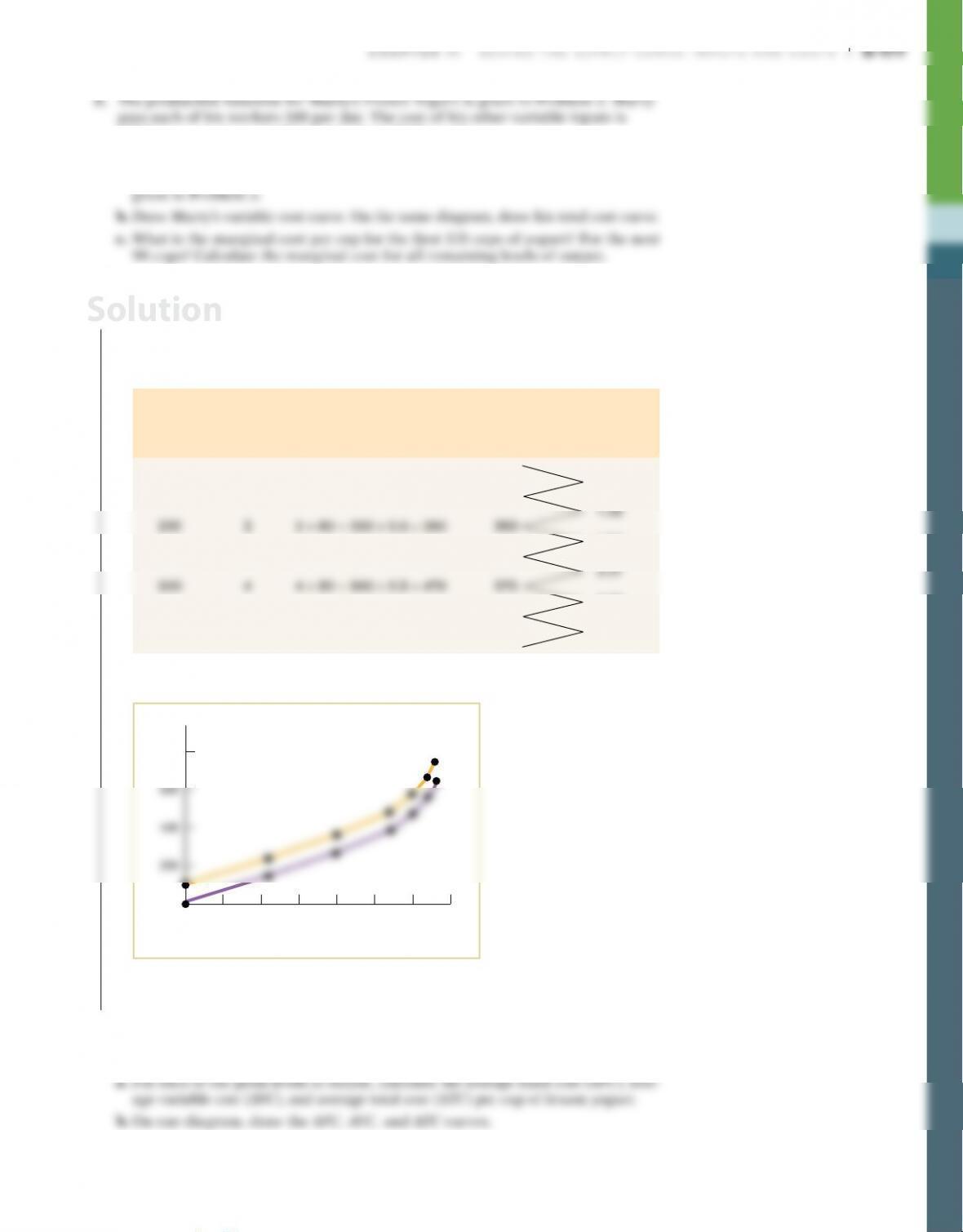
$0.50 per cup of yogurt. His fixed cost is $100 per day.
a. What is Marty’s variable cost and total cost when he produces 110 cups of
yogurt? 200 cups? Calculate variable and total cost for every level of output
3. a. Marty’s variable cost, VC, is his wage cost ($80 per worker per day) and his
other input costs ($0.50 per cup). His total cost, TC, is the sum of the variable
cost and his fixed cost of $100 per day. The answers are given in the accompa-
nying table.
Quantity
of frozen
yogurt
(cups)
Quantity
of labor
(workers) VC TC MC of cup
0 0 $0 $100
$1.23
110 11 × 80 + 110 × 0.5 = 135 235
1.64
270 33 × 80 + 270 × 0.5 = 375 475
4.50
320 55 × 80 + 320 × 0.5 = 560 660
8.50
330 66 × 80 + 330 × 0.5 = 645 745
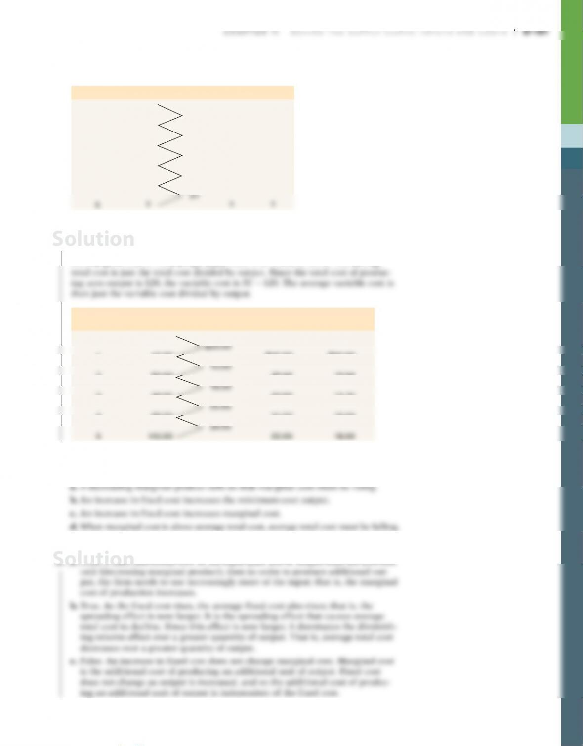
b. The accompanying diagram shows the variable cost and total cost curves.
TC
VC
150100 250200
350
30050
0
$800
Cost
Quantity of frozen yogurt (cups)
c. Marginal cost, MC, per cup of frozen yogurt is shown in the table in part a; it
is the change in total cost divided by the change in quantity of output.
4. The production function for Marty’s Frozen Yogurt is given in Problem 2. The
costs are given in Problem 3.
Solution
S-178 Chapter 11 Behind the Supply Curve: inputS and CoStS
c. What principle explains why the AFC declines as output increases? What princi–
ple explains why the AVC increases as output increases? Explain your answers.
4. a. The average fixed cost, average variable cost, and average total cost per cup of
yogurt are given in the accompanying table. (Numbers are rounded.)
Quantity
of frozen
yogurt (cups) VC TC AFC
of cup AVC of cup ATC of cup
0$0 $100 — — —
110 135 235 $0.91 $1.23 $2.14
320 560 660 0.31 1.75 2.06
330 645 745 0.30 1.95 2.26
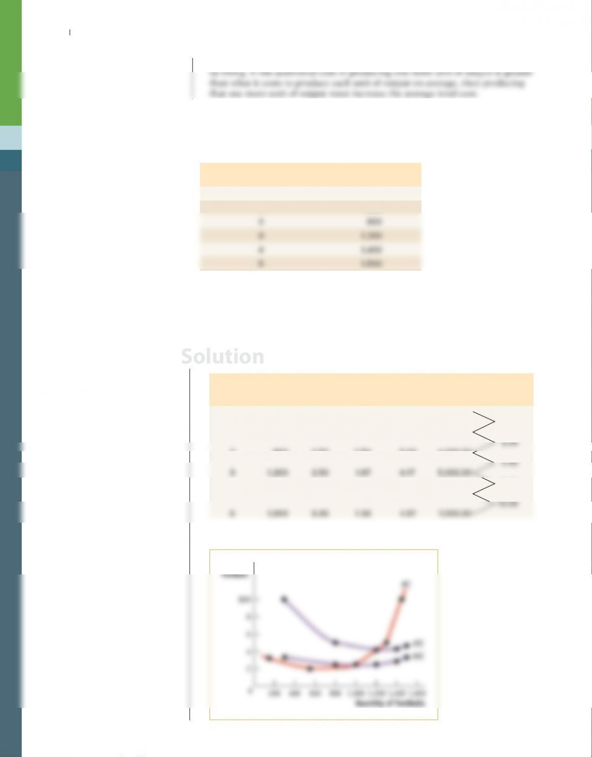
b. The accompanying diagram shows the AFC, AVC, and ATC curves.
150100 250200 350300
0
2.00
0.50
Cost
of
cup
Quantity of frozen yogurt (cups)
ATC
AFC
AVC
5. Labor costs represent a large percentage of total costs for many firms. Accord-
ing to data from the Bureau of Labor Statistics, U.S. labor costs were up 2.0% in
2015, compared to 2014.
a. When labor costs increase, what happens to average total cost and marginal
cost? Consider a case in which labor costs are only variable costs and a case in
which they are both variable and fixed costs.
An increase in labor productivity means each worker can produce more output.
Solution
Chapter 11 Behind the Supply Curve: inputS and CoStS S-179
b. When productivity growth is positive, what happens to the total product curve
and the marginal product of labor curve? Illustrate your answer with a diagram.
c. When productivity growth is positive, what happens to the marginal cost
curve and the average total cost curve? Illustrate your answer with a diagram.
5. a. When labor costs are a variable cost but not a fixed cost, an increase in labor
costs leads to an increase in both average total cost and marginal cost. When
labor costs are a variable cost and a fixed cost, the result is the same: both the
average total cost and the marginal cost increase.
b. When productivity growth is positive, any given quantity of labor can produce
more output, causing the total product curve to shift upward. Since each unit
of labor can produce more output, the marginal product of labor will increase
and the marginal product of labor curve will shift upward. In panel (a) of the
accompanying diagram, the upward shift of the total product curve is illus–
trated by the movement from its initial position, TP1, to its new position, TP2. In
panel (b), the upward shift of the marginal product of labor curve is illustrated
by the movement from its initial position, MPL1, to its new position, MPL2.
Quantity
Marginal
product of
Quantity of labor Quantity of labor
MPL1
MPL2
TP1
(b) Marginal Product Curves(a) Total Product Curves
c. When productivity growth is positive, the marginal cost curve and the aver-
age total cost curve will both shift downward, assuming labor costs have not
changed. In the accompanying diagram, the movement of the average total
cost curve is illustrated by the shift from its initial position, ATC1, to its new
position, ATC2. The movement of the marginal cost curve is illustrated by the
shift from its initial position, MC1, to its new position, MC2.
Cost
of
unit
Quantity
MC
1
MC2ATC1
ATC
2
d. Rising labor costs will shift the average total cost and marginal cost curves
upward. Productivity growth will counteract this, shifting the average total
cost and marginal cost curves downward.
Solution
6. Magnificent Blooms is a florist specializing in floral arrangements for weddings,
graduations, and other events. Magnificent Blooms has a fixed cost associated with
space and equipment of $100 per day. Each worker is paid $50 per day. The daily
production function for Magnificent Blooms is shown in the accompanying table.
Quantity of labor
(workers)
Quantity of floral
arrangements
0 0
1 5
414
515
a. Calculate the marginal product of each worker. What principle explains
why the marginal product per worker declines as the number of workers
employed increases?
6. a. MPL, shown in the accompanying table for the five workers, is the change in out–
put resulting from the employment of one additional worker per day. MPL falls
as the quantity of labor increases due to the principle of diminishing returns.
Quantity
of labor
L
(workers)
Quantity
of floral
arrangements
Q
Marginal
product of
labor MPL =
∆Q/∆L (floral
arrangements
per worker)
Variable
cost VC =
number of
workers ë
wage rate
Total cost
TC =
FC + VC
Marginal
cost of floral
arrangement
MC = ∆TC/∆Q
0 0 $0 $100
5$10.00 (= 50/5)
1 5 50 150
316.67 (= 50/3)
312 150 250
150.00 (= 50/1)
515 250 350
Solution
7. You have the information shown in the accompanying table about a firm’s costs.
Complete the missing data.
Quantity TC MC ATC AVC
0 $20 — —
$20
1 ? ? ?
10
2 ? ? ?
16
3 ? ? ?
20
4 ? ? ?
7. The accompanying table contains the complete cost data. The total cost of pro–
ducing one unit of output is the total cost of producing zero units of output plus
the marginal cost of increasing output from 0 to 1, and so forth. The average
Quantity
of output TC MC of unit ATC of unit AVC of unit
0$20.00 — —
140.00 $40.00 $20.00
250.00 25.00 15.00
366.00 22.00 15.33
486.00 21.50 16.50
8. Evaluate each of the following statements. If a statement is true, explain why; if
it is false, identify the mistake and try to correct it.
8. a. True. If each additional unit of the input adds less to output than the previous
Solution
Solution
S-182 Chapter 11 Behind the Supply Curve: inputS and CoStS
d. False. When marginal cost is above average total cost, average total cost must
9. Mark and Jeff operate a small company that produces souvenir footballs. Their
fixed cost is $2,000 per month. They can hire workers for $1,000 per worker per
month. Their monthly production function for footballs is as given in the accom-
panying table.
Quantity of labor
(workers)
Quantity of
footballs
0 0
1300
a. For each quantity of labor, calculate average variable cost (AVC), average fixed
cost (AFC), average total cost (ATC), and marginal cost (MC).
b. On one diagram, draw the AVC, ATC, and MC curves.
c. At what level of output is Mark and Jeff’s average total cost minimized?
9. a. The AVC, AFC, ATC, TC, and MC are given in the accompanying table.
Quantity
of labor
(workers)
Quantity
of
footballs
AVC of
football
AFC of
football
ATC of
football
TC of
football
MC of
football
0 0 — — — $2,000.00
$3.33
1300 $3.33 $6.67 $10.00 3,000.00
2800 2.50 2.50 5.00 4,000.00
5.00
41,400 2.86 1.43 4.29 6,000.00
b. The accompanying diagram shows the AVC, ATC, and MC curves.
200 400 600 800 1,000 1,200 1,400
1,600
0
$10
8
2
Cost of
f
ootball
Quantity of footballs
MC
Solution
10. You produce widgets. Currently you produce four widgets at a total cost of $40.
a. What is your average total cost?
$5. If you do produce that fifth widget, what will your average total cost be?
Has your average total cost increased or decreased? Why?
10. a. Your average total cost is $40/4 = $10 per widget.
b. If you produce one more widget, you are producing five widgets at a total cost
of $40 + $5 = $45. Your average total cost is therefore $45/5 = $9. Your average
c. If you produce one more widget, you are producing five widgets at a total cost
11. In your economics class, each homework problem set is graded on the basis of a
maximum score of 100. You have completed 9 out of 10 of the problem sets for
the term, and your current average grade is 88. What range of grades for your
10th problem set will raise your overall average? What range will lower your
overall average? Explain your answer.
11. Any grade for your 10th problem set greater than 88 will raise your overall aver-
age; any grade lower than 88 will lower it. This is the same principle at work as
that for average total cost and marginal cost. If the marginal cost curve (the 10th
grade) is above the average total cost curve (the average over the first 9 grades),
then the average total cost is rising (that is, the average over the 10 sets is greater
than the average over the 9 sets). And if the marginal cost curve (the 10th grade)
Sum of grades for first 9 sets
9
= 88 = Average over first 9 sets
Hence,
So your overall grade—the grade over all 10 problem sets—is
792
10 + Grade for 10th set
10 = Overall average
If your 10th grade is 90, then your overall grade is
which is greater than 88. And if your 10th grade is 86, then your overall grade is
which is less than 88.
Solution
Solution
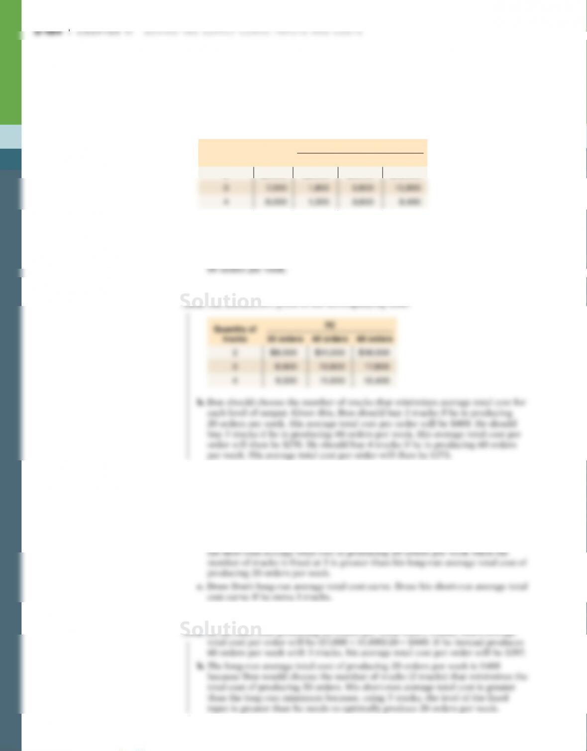
12. Don owns a small concrete-mixing company. His fixed cost is the cost of the
concrete-batching machinery and his mixer trucks. His variable cost is the cost
of the sand, gravel, and other inputs for producing concrete; the gas and main-
tenance for the machinery and trucks; and his workers. He is trying to decide
how many mixer trucks to purchase. He has estimated the costs shown in the
accompanying table based on estimates of the number of orders his company
will receive per week.
Quantity of
trucks
VC
FC 20 orders 40 orders 60 orders
2 $6,000 $2,000 $5,000 $12,000
a. For each level of fixed cost, calculate Don’s total cost for producing 20, 40, and
60 orders per week.
b. If Don is producing 20 orders per week, how many trucks should he purchase
and what will his average total cost be? Answer the same questions for 40 and
13. Consider Don’s concrete-mixing business described in Problem 12. Assume that
Don purchased 3 trucks, expecting to produce 40 orders per week.
a. Suppose that, in the short run, business declines to 20 orders per week. What is
Don’s average total cost per order in the short run? What will his average total
cost per order in the short run be if his business booms to 60 orders per week?
b. What is Don’s long-run average total cost for 20 orders per week? Explain why
Chapter 11 Behind the Supply Curve: inputS and CoStS S-185
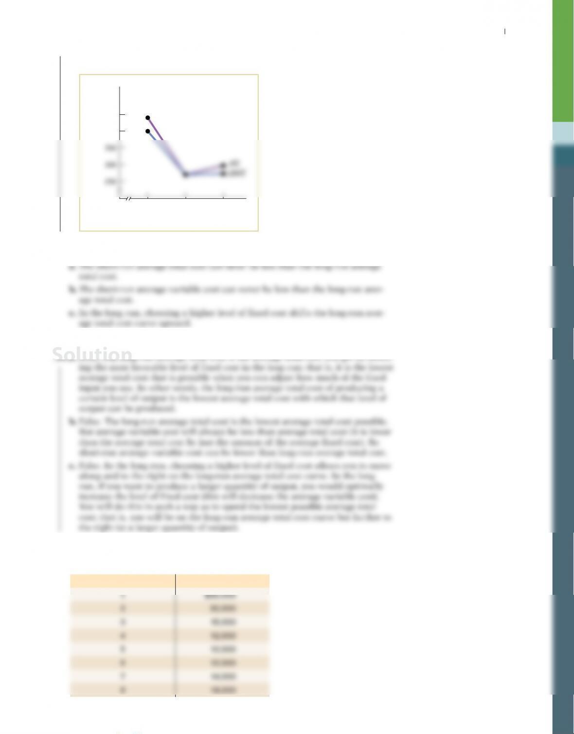
c. The accompanying diagram shows Don’s LRATC and ATC.
$450
400
Cost of
order
S-186 Chapter 11 Behind the Supply Curve: inputS and CoStS
a. For which levels of output does WW experience increasing returns to scale?
b. For which levels of output does WW experience decreasing returns to scale?
c. For which levels of output does WW experience constant returns to scale?
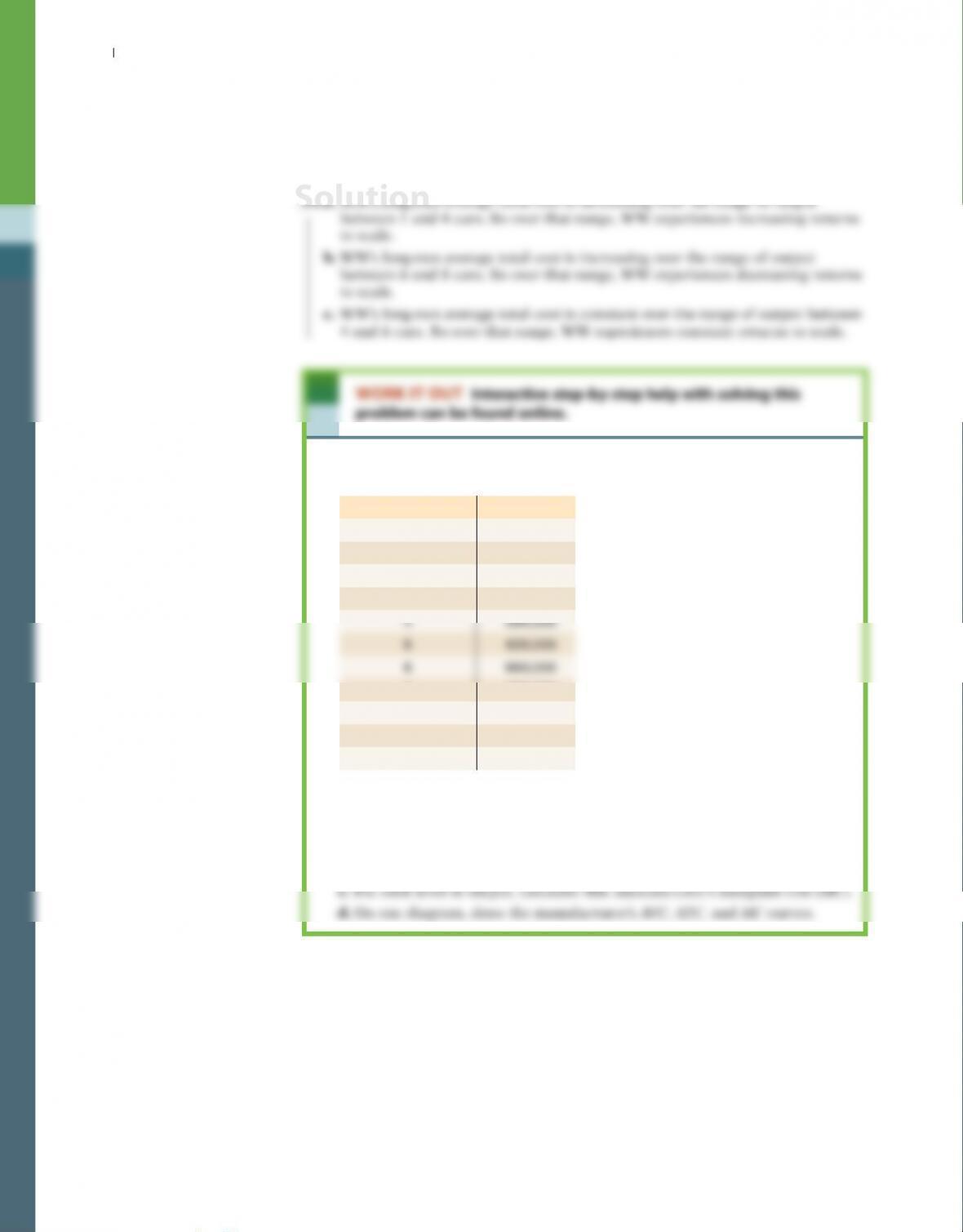
16. The accompanying table shows a car manufacturer’s total cost of producing
cars.
Quantity of cars TC
0$500,000
1540,000
2560,000
3570,000
7720,000
8800,000
9920,000
10 1,100,000
a. What is this manufacturer’s fixed cost?
b. For each level of output, calculate the variable cost (VC). For each level of
output except zero output, calculate the average variable cost (AVC), aver–
age total cost (ATC), and average fixed cost (AFC). What is the minimum-
cost output?
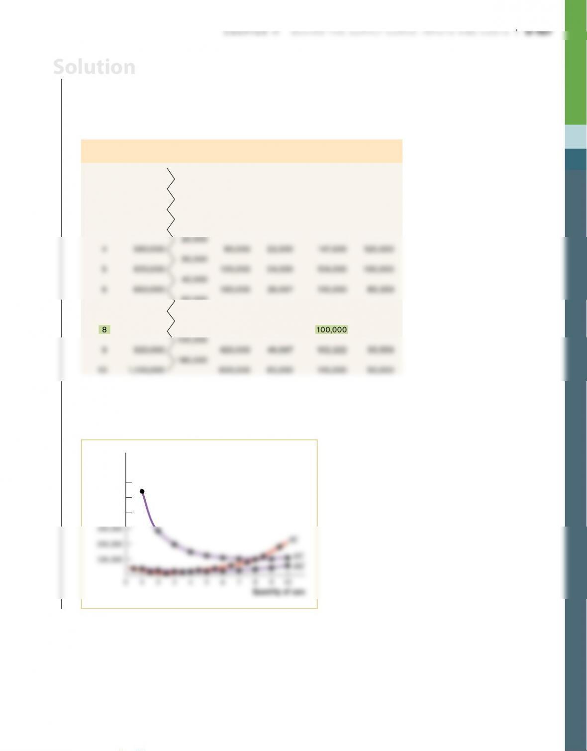
16. a. The manufacturer’s fixed cost is $500,000. Even when no output is produced,
the manufacturer has a cost of $500,000.
b. The accompanying table shows VC, calculated as TC − FC; AVC, calculated
as VC/Q; ATC, calculated as TC/Q; and AFC, calculated as FC/Q. (Numbers
are rounded.) The minimum–cost output is 8 cars, the level at which ATC is
minimized.
Quantity
of cars TC MC of car VC AVC of car ATC of car AFC of car
0$500,000 $0 — — —
$40,000
1540,000 40,000 $40,000 $540,000 $500,000
20,000
2560,000 60,000 30,000 280,000 250,000
10,000
3570,000 70,000 23,333 190,000 166,667
60,000
7720,000 220,000 31,429 102,857 71,429
80,000
8800,000 300,000 37,500 100,000 62,500
c. The table also shows MC, the additional cost per additional car produced. Notice
that MC is below ATC for levels of output less than the minimum–cost output
and above ATC for levels of output greater than the minimum–cost output.
d. The AVC, ATC, and MC curves are shown in the accompanying diagram.
$600,000
500,000
400,000
Cost
of car
Quantity of cars
Solution