
Chapter 10
Classical Business Cycle Analysis:
Market-Clearing Macroeconomics
◼ Learning Objectives
I. Goals of Chapter 10
A. Summarize the real business cycle theory and describe how well it accounts for the business
cycle facts (Sec. 10.1)
II. Notes to Eighth Edition Users
A. We renamed section 10.1 from “Business Cycles in the Classical Model” to “Real Business
Cycle Theory”

Chapter 10 Classical Business Cycle Analysis: Market-Clearing Macroeconomics 209
◼ Teaching Notes
I. The Real Business Cycle Theory (Sec. 10.1)
A. Introduction to real business cycle theory
1. Two key questions about business cycles
a. What are the underlying economic causes?
3. Real business cycle (RBC) theory (Kydland and Prescott)
a. Real shocks to the economy are the primary cause of business cycles
(1) Examples: Shocks to the production function, the size of the labor force, the real
quantity of government purchases, the spending and saving decisions of consumers
(affecting the IS curve or the FE line)
(2) Nominal shocks are shocks to money supply or demand (affecting the LM curve)
b. The largest role is played by shocks to the production function, which the text has called
supply shocks, and RBC theorists call productivity shocks
(1) Examples: Development of new products or production techniques, introduction of
d. Real business cycle theory and the business cycle facts
(1) The RBC theory is consistent with many business cycle facts
(a) If the economy is continuously buffeted by productivity shocks, the theory
Numerical Problem 1 looks at the relationship between real wages and employment over the
business cycle and the issue of whether the labor supply curve should be flat or steep to be
consistent with the data.
(c) The theory correctly predicts procyclical average labor productivity. If booms
weren’t due to productivity shocks, we would expect average labor productivity
210 Abel/Bernanke/Croushore • Macroeconomics, Ninth Edition
(a) But Kydland and Prescott, when using some newer statistical techniques for
calculating the trends in inflation and output, find evidence that the price level is
countercyclical.
Data Application
The “bible” of empirical work on RBC models is by Robert King, Charles Plosser, and Sergio
Rebelo of the University of Rochester, “Production, Growth and Business Cycles: Technical
4. Application: Calibrating the business cycle
a. A major element of RBC theory is that it attempts to make quantitative, not just
qualitative, predictions about the business cycle
b. RBC theorists use the method of calibration to work out a detailed numerical example of
the theory
(1) First they write down specific functions explaining the behavior of people in the
Data Application
The work on calibration has led to a major scientific debate within the economics profession
about how to do empirical work. Economists working on RBC models, led by Prescott, believe
5. Are productivity shocks the only source of recessions?
a. Critics of the RBC theory suggest that except for the oil price shocks of 1973, 1979, and
Chapter 10 Classical Business Cycle Analysis: Market-Clearing Macroeconomics 211
Numerical Problem 6 is a coin-flipping exercise to show that random shocks can lead to big
aggregate movements.
6. Does the Solow residual measure technology shocks?
a. RBC theorists measure productivity shocks as the Solow residual
(1) Named after Robert Solow, the originator of modern growth theory
b. The Solow residual is strongly procyclical in U.S. data
(1) This accords with RBC theory, which says the cycle is driven by productivity shocks
c. But should the Solow residual be interpreted as a measure of technology?
(1) If it’s a measure of technology, it should not be related to factors that don’t directly
d. Measured productivity can vary even if the actual technology doesn’t change
(1) Capital and labor are used more intensively at times
(6) Use this to substitute for Y in Eq. (10.1) to get
(7) So the Solow residual isn’t just A, but depends on uK and uN
(8) Utilization is procyclical, so the measured Solow residual is more procyclical than is
the true productivity term A
(a) Burnside–Eichenbaum–Rebelo evidence on procyclical utilization of capital
e. Conclusion: Changes in the measured Solow residual don’t necessarily reflect changes in
technology
7. Technology shocks may not lead to procyclical productivity
a. Research by Basu and Fernald shows that technology shocks are not closely related to
212 Abel/Bernanke/Croushore • Macroeconomics, Ninth Edition
c. Initially, less capital and labor are needed to produce the same amount of output
d. Later, resources are adjusted and output increases
Theoretical Application
For more on criticisms of the RBC theory and the RBC response to the critics, see the discussion
II. Fiscal Policy Shocks in the Classical Model (Sec. 10.2)
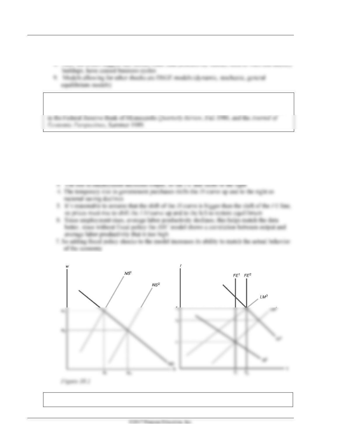
A. The effects of a temporary increase in government expenditures (Figure 10.1; like text
Figure 10.4)
1. The current or future taxes needed to pay for the government expenditures effectively
reduce people’s wealth, causing an income effect on labor supply
2. The increased labor supply leads to a fall in the real wage and a rise in employment
Analytical Problems 2, 3, and 4 deal with various aspects of the classical IS–LM model.

Chapter 10 Classical Business Cycle Analysis: Market-Clearing Macroeconomics 213
B. Should fiscal policy be used to dampen the cycle?
1. Classical economists oppose attempts to dampen the cycle, since prices and wages adjust
quickly to restore equilibrium
4. Also, there may be lags in enacting the correct policy and in implementing it
a. So choosing the right policy today depends on where you think the economy will be in
5. It’s also not clear how much to change fiscal policy to get the desired effect on employment
and output
III. Unemployment in the Classical Model (Sec. 10.3)
A. In the classical model there is no unemployment; people who aren’t working are voluntarily
not in the labor force
C. Classical economists have a more sophisticated version of the model to account for
unemployment
1. Workers and jobs have different requirements, so there is a matching problem
Theoretical Application
D. Davis and Haltiwanger show that there is a tremendous amount of churning of jobs both within
and across industries (text Fig. 10.5)
Data Application
E. But this worker match theory can’t explain all unemployment
1. Many workers are laid off temporarily; there’s no mismatch, just a change in the timing of
work

214 Abel/Bernanke/Croushore • Macroeconomics, Ninth Edition
Data Application
Classical economists believe that unemployment is often affected by institutional factors that
encourage unemployment. Many unemployed workers find jobs once their unemployment
benefits run out, so the government should not (according to classical economists) be very
F. So can the government use fiscal policy to reduce unemployment?
1. Doing so doesn’t improve the mismatch problem
G. Jobless recoveries
1. After each of the last three recessions, employment continued to decline during the recovery,
so the recoveries have come to be known as “jobless recoveries”
2. The previous 5 recessions (before 1990) all featured a sharp rebound in employment as soon
Data Application
Economists have been working hard to come up with good explanations for the jobless
recoveries. Many ideas have been developed but nothing is totally convincing yet. Some

Chapter 10 Classical Business Cycle Analysis: Market-Clearing Macroeconomics 215
Theoretical Application
In most macroeconomic models, including the IS–LM and AD–AS models, the key variables are
economy-wide averages of income, the wage rate, wealth, money holdings, and so on. But some
issues in macroeconomics are better addressed in models in which agents in the model (agents
in terms of the reduced well-being of the agents. In recessions, people who do not lose their jobs
are not affected as much as people who lose their jobs; heterogeneous-agent models can account
for the differential impact on the well-being of different people. In addition, people who lose
their jobs may not be able to borrow, so their consumption spending declines, making them
worse off. Research shows that when people cannot borrow, the costs of business cycles are
significantly larger than if people were able to borrow whenever they lose their jobs, and thus not
have to reduce their spending.
Researchers have also used heterogeneous-agent models to see if they can calibrate the real

216 Abel/Bernanke/Croushore • Macroeconomics, Ninth Edition
IV. Money in the Classical Model (Sec. 10.4)
A. Monetary policy and the economy
Money is neutral in both the short run and the long run in the classical model, because prices
adjust rapidly to restore equilibrium
B. Monetary nonneutrality and reverse causation
1. If money is neutral, why does the data show that money is a leading, procyclical variable?
a. Increases in the money supply are often followed by increases in output
Theoretical Application
In recent years, researchers have found that the RBC model can better match the U.S. data on business
cycles if the model explicitly accounts for household production, which is output produced at home
instead of in a market. Household production includes such goods and services as cooking, child care,
sewing, and food grown in a home garden.
The U.S. national income accounts described in Chapter 2 count mainly the output of
When household production is incorporated into an RBC model, the match between the model
and the data improves, as shown by Jeremy Greenwood of the University of Pennsylvania, Richard
Rogerson of Arizona State University, and Randall Wright of the University of Wisconsin (“Putting
Home Economics into Macroeconomics,” Quarterly Review, Federal Reserve Bank of Minneapolis,
Summer 1993, pp. 2–11). A household-production model has a higher standard deviation of (market)
output than a standard RBC model and more closely matches the U.S. data.

Chapter 10 Classical Business Cycle Analysis: Market-Clearing Macroeconomics 217
Data Application
An early review of empirical work testing the RBC theory of reverse causation is Shaghil
Ahmed, “Does Money Affect Output?” Federal Reserve Bank of Philadelphia Business Review,
3. Why would higher future output cause people to increase money demand?
a. Firms, anticipating higher sales, would need more money for transactions to pay for
Theoretical Application
The early theoretical RBC models did not include a monetary sector at all—they assumed that
money was unimportant for the business cycle. Since then, RBC theorists have been trying
Analytical Problem 5 works out another example of how reverse causation could occur through
firms’ demand for money for transactions and the Fed’s money supply response.
C. The nonneutrality of money: Additional evidence
1. Friedman and Schwartz have extensively documented that often monetary changes have had
an independent origin; they weren’t just a reflection of changes or future changes in
2. More recently, Romer and Romer documented additional episodes of monetary nonneutrality
since 1960
Theoretical Application
For a thorough overview of how money works to affect the economy in various models, see the
3. So money does not appear to be neutral

218 Abel/Bernanke/Croushore • Macroeconomics, Ninth Edition
Numerical Problems 2 and 3 examine price level effects in the classical model.
V. The Misperceptions Theory and the Nonneutrality of Money (Sec. 10.5)
A. Introduction to the misperceptions theory
1. In the classical model, money is neutral since prices adjust quickly
2. But if producers misperceive the aggregate price level, then the relevant aggregate supply
curve in the short run isn’t vertical
a. This happens because producers have imperfect information about the general price level
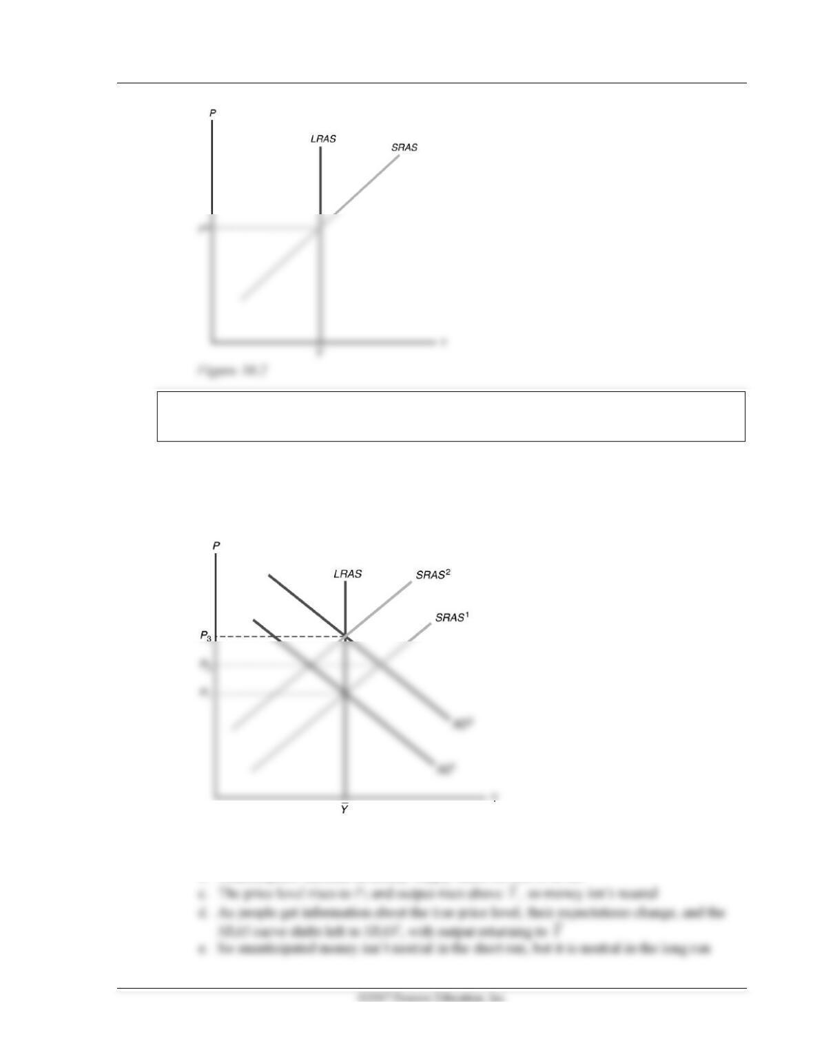
B. The misperceptions theory is that the aggregate quantity of output supplied rises above the full–
employment level
Y
when the aggregate price level P is higher than expected
1. This makes the AS curve slope upward
2. Example: A bakery that makes bread
a. The price of bread is the baker’s nominal wage; the price of bread relative to the general
price level is the baker’s real wage
3. Generalizing this example, if everyone expects prices to increase 5% but they actually
increase 8%, they’ll work more
4. So, an increase in the price level that is higher than expected induces people to work more
Chapter 10 Classical Business Cycle Analysis: Market-Clearing Macroeconomics 219
Analytical Problem 1 contracts the effects of a change in the future marginal product of capital in
an RBC model to that in a misperceptions model.
C. Monetary policy and the misperceptions theory
1. Because of misperceptions, unanticipated monetary policy has real effects; but anticipated
monetary policy has no real effects because there are no misperceptions
2. Unanticipated changes in the money supply (Figure 10.3; like text Figure 10.8)
Figure 10.3
a. Initial equilibrium where AD1 intersects SRAS1 and LRAS
b. Unanticipated increase in money supply shifts AD curve to AD2

220 Abel/Bernanke/Croushore • Macroeconomics, Ninth Edition
3. Anticipated changes in the money supply
a. If people anticipate the change in the money supply and thus in the price level, they
Data Application
Do the data support the misperceptions theory? Robert Barro, “Unanticipated Money,
D. Rational expectations and the role of monetary policy
1. The only way the Fed can use monetary policy to affect output is to surprise people
2. But people realize that the Fed would want to increase the money supply in recessions and
decrease it in booms, so they won’t be fooled
Numerical Problems 4 and 8 look at the misperceptions theory and unanticipated compared to
anticipated changes in the money supply.
6. Propagating the effects of unanticipated changes in the money supply
a. It doesn’t seem like people could be fooled for long, since money supply figures are
c. Example of propagation: The behavior of inventories
(1) Firms hold a normal level of inventories against their normal level of sales
(2) An unanticipated increase in the money supply increases sales

Chapter 10 Classical Business Cycle Analysis: Market-Clearing Macroeconomics 221
Theoretical Application
Although the text presents the theories in the reverse order, the misperceptions theory came first
(being developed in the 1970s) and the RBC theory came later (in the 1980s). Many classical
economists moved away from the misperceptions theory because they weren’t convinced by its
E. In touch with data and research: Are price forecasts rational?
1. Economists can test whether price forecasts are rational by looking at surveys of people’s
expectations
Data Application
If you examine a survey of forecasters, like the Livingston Survey, you’ll see that the forecasters
made very bad forecasts of inflation around 1973 to 1974 and again around 1979 to 1980. Both
4. Many statistical studies suggest that people don’t have rational expectations
5. But people who answer surveys may not have a lot at stake in making forecasts, so couldn’t
be expected to produce rational forecasts

222 Abel/Bernanke/Croushore • Macroeconomics, Ninth Edition
Data Application
The survey used by Keane and Runkle was begun by Victor Zarnowitz of the University of
Chicago in 1968 and was run by the American Statistical Association and National Bureau of