304 Chapter 10
P10.4 Long-run Firm Supply. The retail market for unleaded gasoline is fiercely price
competitive. Consider the situation faced by a typical gasoline retailer when the local
market price for unleaded gasoline is $1.80 per gallon and total cost (TC) and marginal
cost (MC) relations are:
TC = $40,000 + $1.64Q + $0.0000001Q2
MC =
TC/
Q = $1.64 + $0.0000002Q
and Q is gallons of gasoline. Total costs include a normal profit.
A. Using the firm’s marginal cost curve, calculate the profit-maximizing long-run
supply curve for a typical retailer
B. Calculate the average total cost curve for a typical gasoline retailer, and verify
that average total costs are less than price at the optimal activity level.
P10.4 SOLUTION
A. The marginal cost curve constitutes the long-run supply curve for firms in perfectly
competitive markets if price is greater than average total cost. Because P = MR, the
B. The average total cost curve is determined by dividing total cost by output:
Competitive Markets 305
long-run equilibrium.
P10.5 Short-run Firm Supply. Farm Fresh, Inc., supplies sweet peas to canneries located
throughout the Mississippi River Valley. Like many grain and commodity markets, the
market for sweet peas is perfectly competitive. With $250,000 in fixed costs, the
company’s total and marginal costs per ton (Q) are:
TC = $250,000 + $200Q + $0.02Q2
MC =
TC/
Q = $200 + $0.04Q
A. Calculate the industry prices necessary to induce short-run quantities supplied by
the firm of 5,000, 10,000, and 15,000 tons of sweet peas. Assume that MC > AVC
at every point along the firm’s marginal cost curve and that total costs include a
normal profit.
B. Calculate short-run quantities supplied by the firm at industry prices of $200,
$500, and $1,000 per ton.
P10.5 SOLUTION
A. The marginal cost curve constitutes the short-run supply curve for firms in perfectly
competitive industries provided price exceeds average variable cost. Because P = MR,
306 Chapter 10
B. When quantity is expressed as a function of price, the firm’s supply curve can be
written:
Q = -5,000 + 25P
Therefore, at:
P10.6 Short-run Market Supply. New England Textiles, Inc., is a medium-sized manufacturer
of blue denim that sells in a perfectly competitive market. Given $25,000 in fixed costs,
the total cost function for this product is described by:
TC = $25,000 + $1Q + $0.000008Q2
MC = ∂TC/∂Q = $1 + $0.000016Q
where Q is square yards of blue denim produced per month. Assume that MC > AVC at
every point along the firm’s marginal cost curve, and that total costs include a normal
profit.
A. Derive the firm’s supply curve, expressing quantity as a function of price.
B. Derive the market supply curve if New England Textiles is one of 500 competitors.
C. Calculate market supply per month at a market price of $2 per square yard.
P10.6 SOLUTION
Competitive Markets 307
A. The perfectly competitive firm will supply output so long as it is profitable to do so.
Because P = MR in perfectly competitive markets, the firm supply curve is given by the
relation:
B. If the company is one of 500 such competitors, the industry supply curve is found by
simply multiplying the firm supply curve derived in part A by 500. This is equivalent to
When price is expressed as a function of quantity:
P10.7 Long-run Competitive Firm Supply. The Hair Stylist, Ltd., is a popular-priced
hairstyling salon in College Park, Maryland. Given the large number of competitors,
the fact that stylists routinely tailor services to meet customer needs, and the lack of
entry barriers, it is reasonable to assume that the market is perfectly competitive and
308 Chapter 10
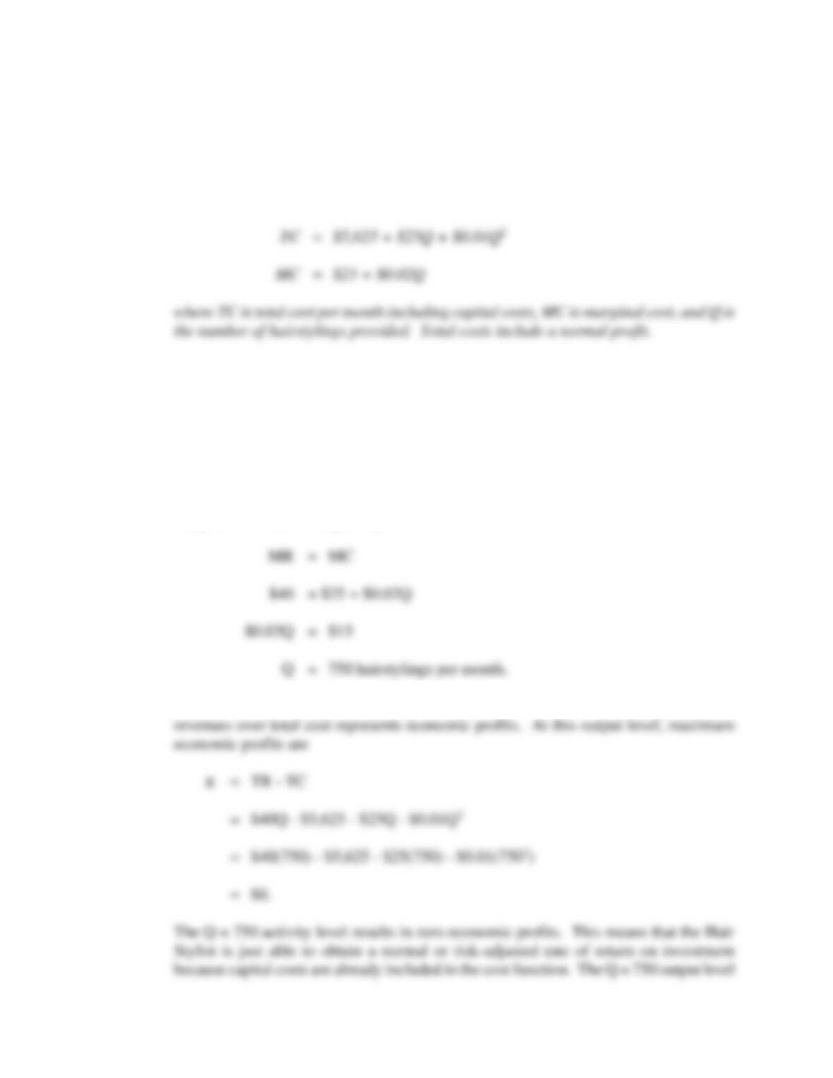
that the average $40 price equals marginal revenue, P = MR = $40. Furthermore,
assume that the firm’s operating expenses are typical of the 100 firms in the local market
and can be expressed by the following total and marginal cost functions:
A. Calculate the firm’s profit-maximizing output level.
B. Calculate the firm’s economic profits at this activity level. Is this activity level
sustainable in the long run?
P10.7 SOLUTION
A. The optimal output level can be determined by setting marginal revenue equal to
marginal cost and solving for Q:
B. Because the cost of capital is already included in the total cost function, any excess of
Competitive Markets 309
P10.8 Competitive Market Equilibrium. Dozens of Internet web sites offer quality auto parts
for the replacement market. Their appeal is obvious. Price-conscious shoppers can
often obtain up to 80% discounts from the prices charged by original equipment
manufacturers (OEMs) for such standard items as wiper blades, air filters, oil filters,
and so on. With a large selection offered by dozens of online merchants, the market for
standard replacement parts is vigorously competitive. Assume that market demand and
supply conditions for windshield wiper blades can be described by the following
relations:
where Q is millions of replacement wiper blades and P is price per unit.
A. Graph the market demand and supply curves.
P10.8 SOLUTION
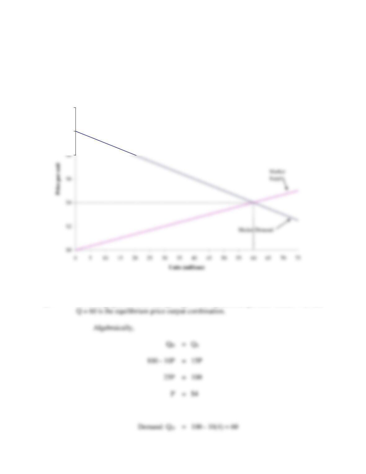
A.
310 Chapter 10
B. From the graph, it is clear that QD = QS = 60 at a price of $4 per unit. Thus, P = $4 and
Both demand and supply equal 60 because:
Demand and Supply Conditions for
Replacement Windshield Wiper Blades
$10
$12
Competitive Markets 311
P10.9 Dynamic Competitive Equilibrium. Wal-Mart and other movie DVD retailers,
including online vendors like amazon.com, employ a two-step pricing policy. During the
first six months following a theatrical release, movie DVD buyers are wiling to pay a
premium for new releases. Total and marginal revenue relations for a typical newly
released movie DVD are given by the following relations:
TR = $28Q – $0.0045Q2
MR = ∂TC/∂Q = $28 – $0.009Q
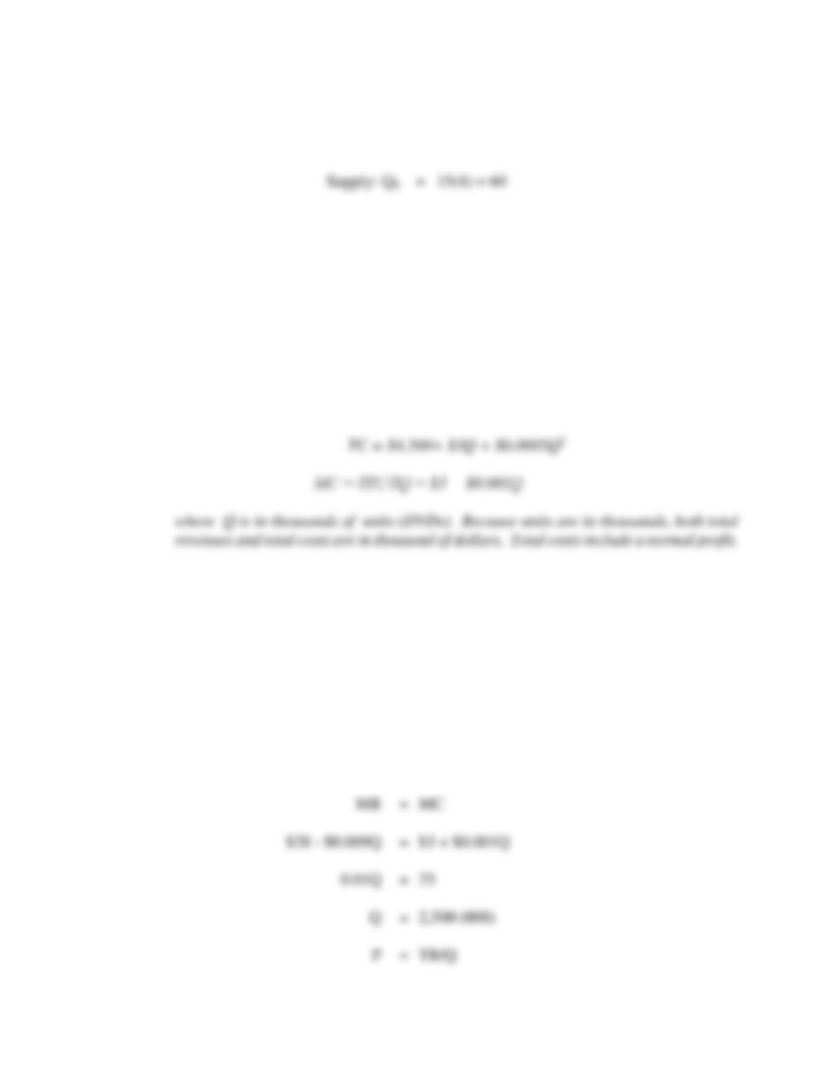
Total cost (TC) and marginal costs (MC) for production and distribution are:
A. Use the marginal revenue and marginal cost relations given above to calculate
DVD output, price, and economic profits at the profit-maximizing activity level for
new releases.
B. After six months, price-sensitive DVD buyers appear willing to pay no more than
$6 per DVD. Calculate the equilibrium price-output activity level in this situation.
Is this a stable equilibrium?
P10.9 SOLUTION
A. Set MR = MC to find the profit-maximizing activity level:
312 Chapter 10
B. In a perfectly competitive industry, P = MR = MC in equilibrium. Thus, six months
P10.10 Stable Competitive Equilibrium. Bada Bing, Ltd., supplies standard 256 MB-RAM
chips to the U.S. computer and electronics industry. Like the output of its competitors,
Bada Bing’s chips must meet strict size, shape, and speed specifications. As a result, the
chip-supply industry can be regarded as perfectly competitive. The total cost and
marginal cost functions for Bada Bing are:
Competitive Markets 313
where Q is the number of chips produced. Total costs include a normal profit.
A. Calculate Bada Bing’s optimal output and profits if chip prices are stable at $60
each.
B. Calculate Bada Bing’s optimal output and profits if chip prices fall to $30 each.
C. If Bada Bing is typical of firms in the industry, calculate the firm’s long-run
equilibrium output, price, and economic profit levels.
P10.10 SOLUTION
A. Because the industry is perfectly competitive, P = MR = $60. Set MR = MC to find the
Therefore,
314 Chapter 10
C. In equilibrium, P = AC and MR = MC at the point where average cost is minimized. To
find the point of minimum average costs set MC = AC, and solve for Q:
Competitive Markets 315
316 Chapter 10
CASE STUDY FOR CHAPTER 10
Profitability Effects of Firm Size for DJIA Companies
Does large firm size, pure and simple, give rise to economic profits? This question has long been a
source of great interest in both business and government, and the basis for lively debate over the
years. Economic theory states that large relative firm size within a given economic market gives rise
Still, without a doubt, the profitability effect of large firm size is a matter of significant
business and public policy interest. Ranking among the largest corporations in the United States is
a matter of significant corporate pride for employees, top executives, and stockholders. Sales and
profit levels achieved by such firms are widely reported and commented upon in the business and
popular press. At times, congressional leaders have called for legislation that would bar mergers
among giant companies on the premise that such combinations create monolithic giants that impair
competitive forces. Movements up and down lists of the largest corporations are chronicled,
studied, and commented upon. It is perhaps a little known fact that, given the dynamic nature of
change in the overall economy, few companies are able to maintain, let alone enhance, their relative
position among the largest corporations over a 5- to 10-year period. With an annual attrition rate
of 6% to 10% among the 500 largest corporations, it indeed appears to be “slippery” at the top.
To evaluate the link, if any, between profitability and firm size, it is interesting to consider
the data contained in Table 1.1 on the corporate giants found within the Dow Jones Industrial
Average (DJIA). These are profit and size data on 30 of the largest and most successful
Table 1.1 shows profitability as measured by net income, and two standard measures of firm
size. Sales revenue is perhaps the most common measure of firm size. From an economic
Competitive Markets 317
perspective, sales is an attractive measure of firm size because it is not susceptible to accounting
manipulation or bias, nor is it influenced by the relative capital or labor intensity of the enterprise.
When size is measured by sales revenue, measurement problems tied to inflation, replacement cost
errors, and so on, are minimized. Another popular measure of firm size is net worth, or the book
value of stockholders’ equity, defined in accounting terms as total assets minus total liabilities.
Stockholders’ equity is a useful measure of the total funds committed to the enterprise by
stockholders through paid in capital plus retained earnings.
The simplest means for studying the link between profitability and firm size is to compare
profits and firm size, when size is measured using sales and stockholders’ equity. However, it is
The effects of firm size on profits and firm size on profit rates among the corporate giants
found among the DJIA are shown in Table 10.2.
A. Based upon the findings reported in Table 10.2, discuss the relation between firm size
and profitability, and the link, if any, between firm size and profit rates. In general, does
large firm size increase profitability?
C. What other important factors might be included in a more detailed study of the
determinants of corporate profitability?
CASE STUDY SOLUTION
A. Using a simple ordinary least squares regression approach to investigating the firm size-
profit rate relation, there is no apparent profit advantage to large firm size. These results
318 Chapter 10
B. Profits and profit rates vary on a year-by-year basis for the corporate giants found within
the DJIA. Wal-Mart, Exxon and GM are commonly found among the very largest
C. A number of other important factors might be considered in a more detailed study of the
determinants of profitability for corporate giants. For example, rapid firm growth can be