154
CHAPTER 10
General Equilibrium and
Welfare
A. Summary
This chapter provides a very elementary introduction to general equilibrium
theory. It begins by showing why taking a general equilibrium approach may
be necessary to address some important economic questions and then pro-
ceeds to build a simply model of two markets. That model (drawn primarily
from the graphical approach to international trade theory) generalizes “sup-
ply” by using the production possibility frontier and “demand” by using a
typical person’s indifference curve. An advantage of this approach is to
stress that the economic “problem” is how to make the best (utility–
maximizing) use of scarce resources.
B. Lecture and Discussion Suggestions
Repeating the development of the general equilibrium model in this chapter
in lecture would probably be quite dull. Hence, it may better to assume that
students have understood the development in the text and just use the model
to illustrate some results. One approach that seems to work well is to use
Chapter 12: General Equilibrium and Welfare
155
croeconomics Classroom” (Journal of Economic Education, Summer, 2009.
Pages 297-314) provides a nice such introduction. But there are many other
possibilities that could be used.
Discussions of general equilibrium might focus on “what more did you
learn by using these models?” For example, students may find that tax inci-
C. Glossary Entries in the Chapter
• Contract Curve
• Economically Efficient Allocation of Resources
• Equity
• Externality
SOLUTIONS TO CHAPTER 10 PROBLEMS
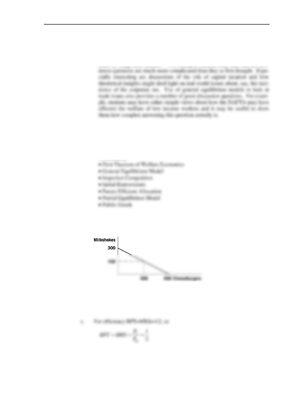
10.1 a. The production possibility frontier for M and C is shown as:
b. If people want M = ½ C and technology requires C + 2M = 600, then C +
2(1/2C) = 600.
2C = 600 or C = 300. M = 150.
Chapter 12: General Equilibrium and Welfare
156
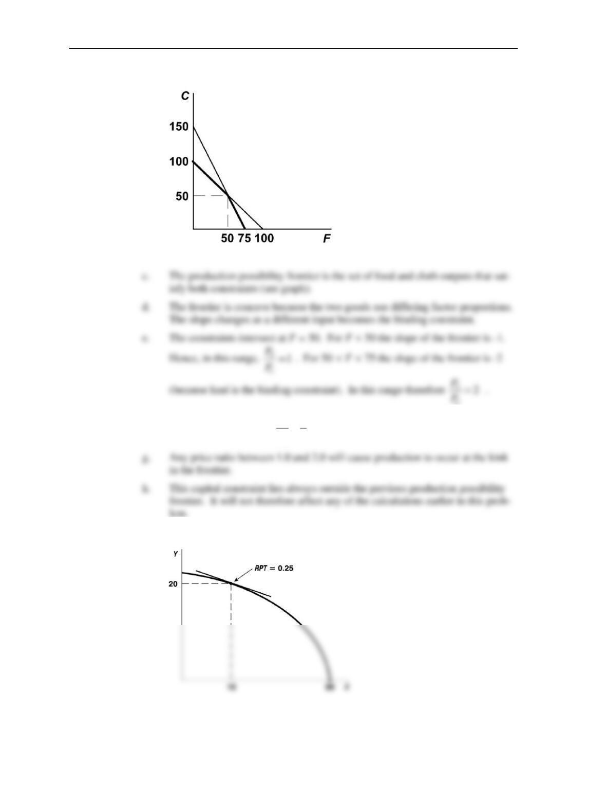
10.2 a. See Graph
b. See Graph
C
f. With these preferences,
5
4
F
C
P
P=
.
10.3 a. The frontier is a quarter ellipse:
Chapter 12: General Equilibrium and Welfare
157
b. If
22
2 , 2(2 ) 900Y X X X= + =
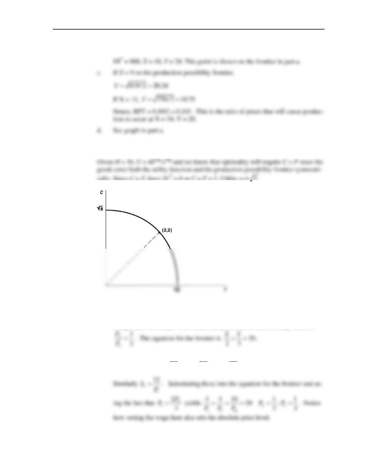
10.4 Since
8
FC
LL+=
. the production possibility frontier is F2 + C2 = 8
cally. Since C = F, have 2C2 = 8 or C = F = 2. Utility = 4
2.
10.5 a. Given the production conditions, the production possibility frontier will be a
straight line with slope – 3/2. Hence the price ratio in this economy must be
b. Using the hint,
3 5 8
S J T
X X X
X X X
P P P
= = =
Chapter 12: General Equilibrium and Welfare
158
10.6 a. For region A the production possibility frontier is
22
100
XY+=
. For region
10.7 a.
12
10 5UU==
.
10.8 a. The total value of transactions is 20w. So, money supply = 60 = money de-
mand = 5w. So w = 12 (earlier we assumed
10w=
) So the absolute prices
Chapter 12: General Equilibrium and Welfare
159
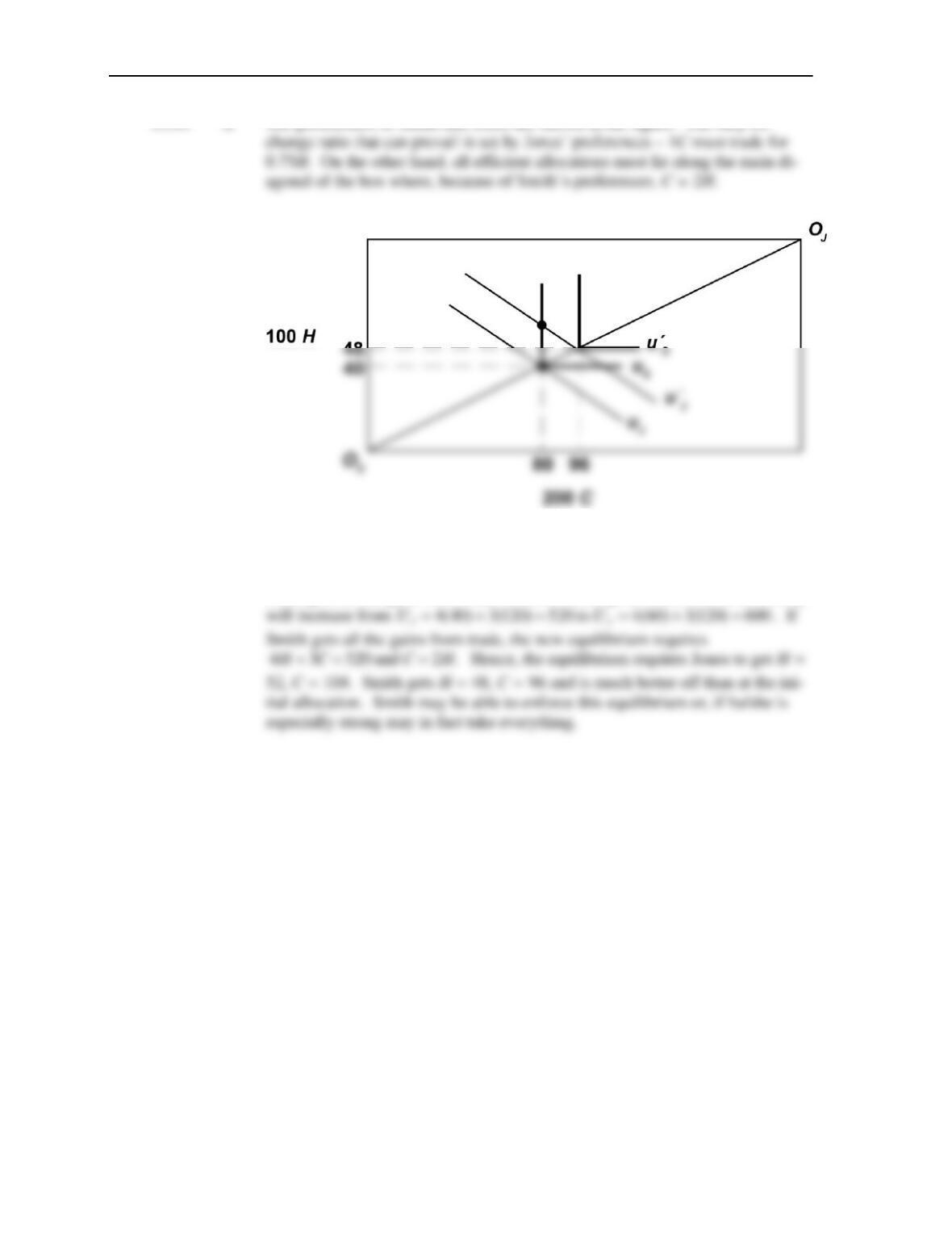
10.9 a-c. See Graph
d. As before, efficient points are the tangencies of the isoquants.
e. The production possibility frontier shows the maximum amount of Y that can
f.
(i) The production possibility frontier is a single point where X gets all labor
input, Y gets all capital input.
Chapter 12: General Equilibrium and Welfare
160
10.10 a. The preferences of Smith and Jones are shown in the figure. The only ex-
b. This is an equilibrium – the allocation lies on the contract curve and any trade
would make at least one person worse off.
c. Now the initial position is off the contract curve. Smith has 20“extra” H. If
Jones gets all the gains from trade because Smith gives these to him/her, utility