
Chapter 10 Classical Business Cycle Analysis: Market-Clearing Macroeconomics 223
◼ Additional Issues for Classroom Discussion
1. Do Wages Adjust to Clear the Labor Market?
One of the key assumptions of classical macroeconomic theory is that wages adjust rapidly to bring about
equilibrium in the labor market in a relatively short period of time. Is this a reasonable assumption?
Some economists look at the labor-market statistics, which show large swings in unemployment and
not much change in wages over the business cycle. They believe this indicates sluggish wage adjustment,
2. Are People’s Inflation Forecasts Rational?
When the misperceptions theory was developed in the late 1970s, a number of economists began testing
people’s forecasts to see how rational they were. The theory implies that on average, people should not
make systematic errors in forecasting. Of special importance are people’s forecasts of inflation, since
these affect the aggregate supply curve.

224 Abel/Bernanke/Croushore • Macroeconomics, Ninth Edition

Chapter 10 Classical Business Cycle Analysis: Market-Clearing Macroeconomics 225
◼ Answers to Textbook Problems
Review Questions
1. The main feature of the classical IS–LM model that distinguishes it from the Keynesian IS–LM model
is the classical model’s assumption that prices adjust quickly to restore equilibrium. Keynesians
2. The two main components of any theory of the business cycle are (1) a specification of the types of
shocks or disturbances that are believed to be the most important in affecting the economy and (2) a
3. A real shock is a disturbance to the real side of the economy that affects the IS curve or the FE line.
A nominal shock is a disturbance to money supply or money demand that affects the LM curve. Real
4. RBC theory is successful at explaining that employment is procyclical, that average labor productivity
5. The Solow residual is the most common measure of productivity shocks. It is strongly procyclical,
rising in expansions and declining in contractions. The Solow residual changes when total factor
productivity changes, when capital utilization changes, and when labor utilization changes.
6. The increase in government purchases does not affect labor demand, but causes an increase in labor
supply at any given real wage. This occurs because workers are poorer due to the current or future
taxes they must pay to finance the increased government spending. Since labor demand is unchanged

226 Abel/Bernanke/Croushore • Macroeconomics, Ninth Edition
7. Reverse causation means that expected future increases in output cause increases in the current
money supply, and expected future decreases in output cause decreases in the current money supply.
8. According to the misperceptions theory, an increase in the price level fools producers of goods into
producing more, because they are unable to tell whether the increase in prices is a relative price
9. In the classical model, money is neutral in both the short run and the long run. This is modified in the
10. Rational expectations mean that the public’s forecasts of various economic variables are based on
Chapter 10 Classical Business Cycle Analysis: Market-Clearing Macroeconomics 227
Numerical Problems
1. (a) Labor supply is given by the equation NS = 45 + 0.1w. Before the shock, labor demand is
determined by the equation w = 1.0(100 − N). Setting labor supply equal to labor demand by
substituting the labor demand equation into the labor supply equation gives N = 45 + 0.1 w =
(c) If the real wage is only slightly procyclical, then a flat labor supply curve, as in part (b) is
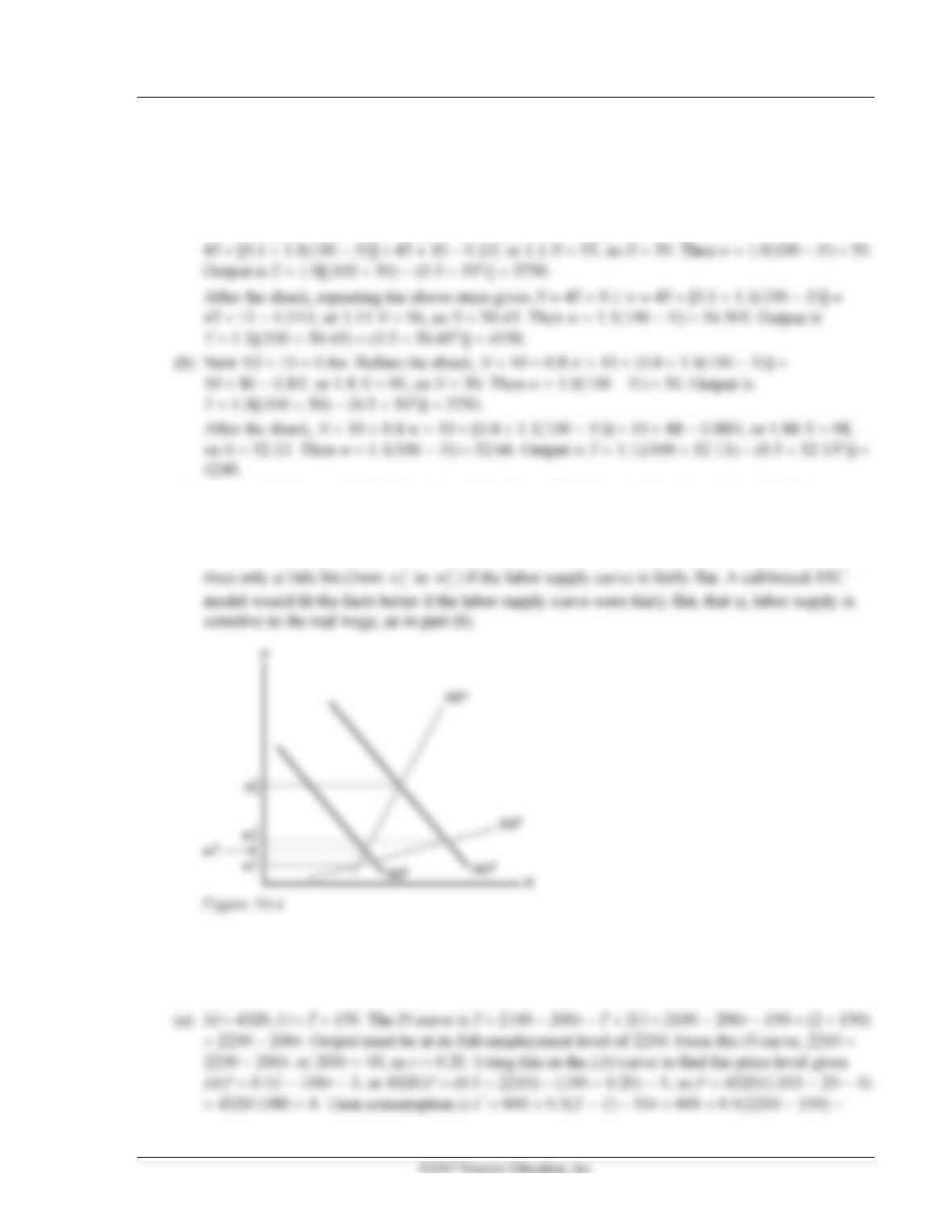
necessary, rather than a steep labor supply curve as in part (a). Figure 10.4 illustrates the
difference in slopes of the two labor supply curves. When labor demand increases from ND1 to
ND2, the real wage rises a lot (from
1
a
w
to
2
a
w
) with a steep labor supply curve, but the real wage
1
b
w
2
b
w
2. The IS curve gives Y = C + I + G = 600 + 0.5(Y − T) − 50r + 450 − 50r + G = 1050 − 100r + 0.5Y −
0.5T + G, or 0.5Y = 1050 − 100r − 0.5T + G, or Y = 2100 − 200r − T + 2G. The LM curve gives
M/P = L = 0.5Y − 100i = 0.5Y − 100(r +
) = 0.5Y − 100(r + 0.05) = 0.5Y − 100r − 5.

228 Abel/Bernanke/Croushore • Macroeconomics, Ninth Edition
3. The IS curve is found by setting desired saving equal to desired investment. Desired saving is
Sd = Y − Cd − G = Y − [250 + 0.5(Y − T) − 500r] − G. Setting Sd = Id gives Y − [250 + 0.5(Y − T) − 500r]
− G = 250 − 500r, or Y = 1000 − 2000r + 2G − T. The LM curve is M/P = L = 0.5Y − 500i = 0.5Y −
500(r +
e) = 0.5Y − 500r.
Consumption is C = 250 + 0.5(Y − T) − 500r = 250 + 0.5(1000 − 200) − (500 0.10) = 600.
Investment is I = 250 − 500r = 250 − (500 0.10) = 200.
(b) Following the same steps as above, with M = 9000 instead of 7650, gives the aggregate demand
curve AD: Y = 400 + (12,000/P). With Y = 1000, this gives P = 20. Nothing has changed in the IS
equation, so it still gives r = 0.10. And nothing has changed in either the consumption or
4. AD: Y = 300 + 30(M/P), AS: Y = 500 + 10(P – Pe), M = 400.
(a) Pe = 60. Setting AD = AS to eliminate Y, we get 300 + 30(M/P) = 500 + 10(P − Pe). Plugging in
the values of M and Pe gives 300 + (30 400/P) = 500 + 10(P − 60), or 300 + (12,000/P) = 500 +
Chapter 10 Classical Business Cycle Analysis: Market-Clearing Macroeconomics 229
5. (a) To find the Solow residual, use the equation for the production function, dividing through to
solve for A: A = Y/K0.3N0.7. Assuming there’s no change in utilization rates, this is the measured
Solow residual. Given that equation, plugging in the values for Y, K, and N, gives the Solow
residual as 1.435 in 2006 and 1.507 in 2007. The growth rate of the Solow residual is
[(1.507/1.435) − 1] 100% = 5.0%.
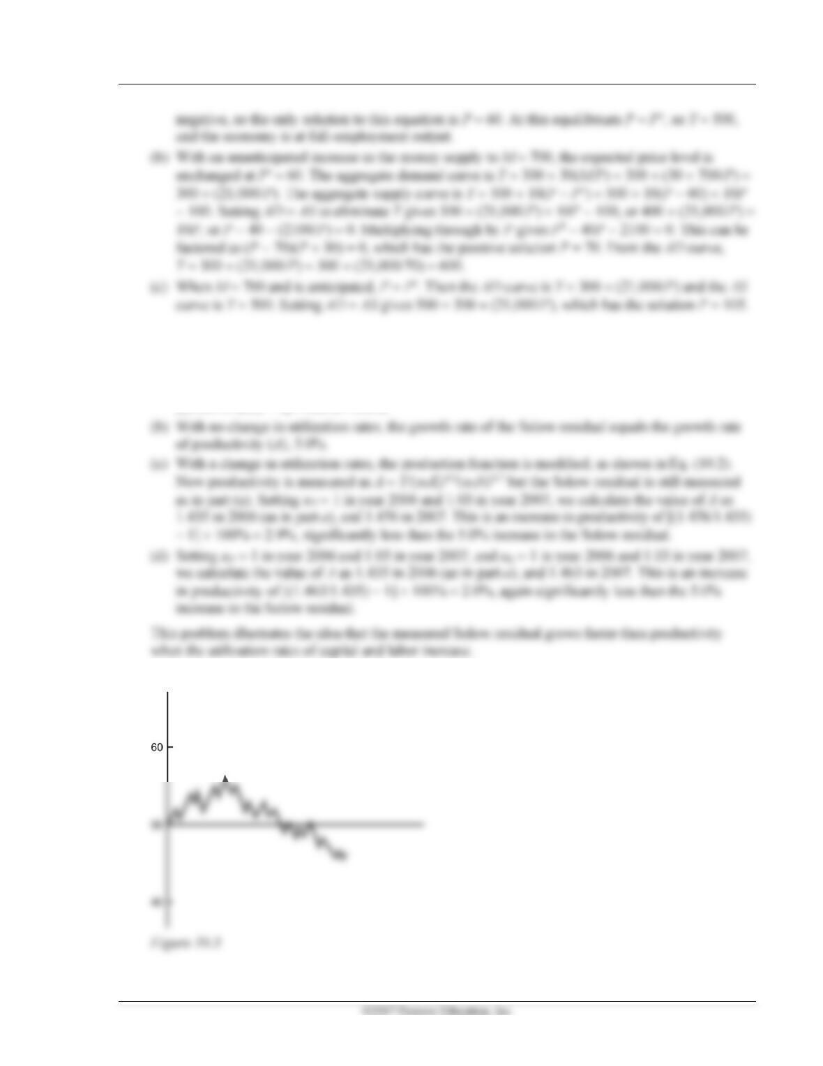
6. An example is shown in Figure 10.5. There are several long cycles in output.

230 Abel/Bernanke/Croushore • Macroeconomics, Ninth Edition
7. (a) With an unemployment rate of 5%, there are initially 5 million unemployed and 95 million
employed. Since 1% of the employed become unemployed, 95 million 0.01 = 950,000 move
from employment to unemployment each month. Since 19% of the unemployed become
employed, 5 million 0.19 = 950,000 from unemployment each month. Since the same number
8. (a)
IS = 2.47,
IS = 0.0004,
LM = 0,
LM = 0.001, lr = 500, b = 100.
(b) Y = [2.47 + 88,950/(P 500)]/(.0004 + .001) = (2.47 + 177.9/P)/.0014
(c) Y = 6000 + 100P − 2915 = 3085 + 100P; use this in the AD curve to eliminate Y.

Chapter 10 Classical Business Cycle Analysis: Market-Clearing Macroeconomics 231
Analytical Problems
1. (a) The increase in MPKf leaves aggregate supply unchanged, since expected future labor income
and expected future wages are unchanged. But aggregate demand increases, because firms
increase investment, shifting the IS curve up and to the right. There is no shift in either the LM
curve or the FE line.
2. (a) In the case of a permanent increase in government purchases, the income effect on labor supply,
which arises because the present value of taxes increases to pay for the added government
spending, is much higher than in the case of a temporary increase in government spending. So
workers increase their labor supply more when the government spending change is permanent
than when it is temporary.
232 Abel/Bernanke/Croushore • Macroeconomics, Ninth Edition

Chapter 10 Classical Business Cycle Analysis: Market-Clearing Macroeconomics 233
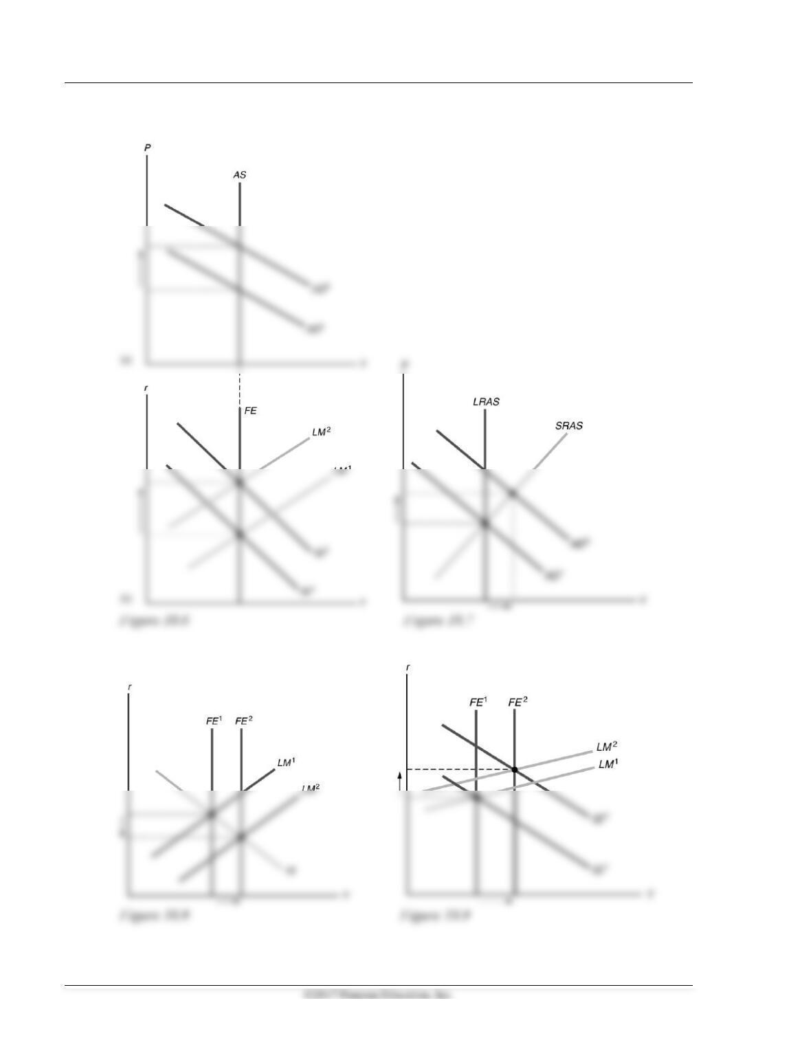
3. The temporary increase in government purchases causes an income effect that increases workers’
labor supply. This results in an increase in the full-employment level of output from FE1 to FE2 in
Figure 10.10. The increase in government purchases also shifts the IS curve up and to the right from
IS1 to IS2, as it reduces national saving. Assuming that the shift up of the IS curve is so large that it
intersects the LM curve to the right of the FE line, the price level must rise to get back to equilibrium
Figure 10.11 shows the impact on the labor market. Labor supply shifts from NS1 to NS2, leading to a
decline in the real wage and a rise in employment. Average labor productivity declines, since
employment rises while capital is fixed. Investment declines, since the real interest rate rises.
To summarize, in response to a temporary increase in government purchases, output, the real interest
rate, the price level, and employment rise, while average labor productivity and investment decline.
(a) The business cycle fact is that employment is procyclical. The model is consistent with this fact,

234 Abel/Bernanke/Croushore • Macroeconomics, Ninth Edition
(c) The business cycle fact is that average labor productivity is procyclical. The model is
inconsistent with this fact, since it shows a decline in average labor productivity when
4 . The temporary wage tax has a small income effect but a large substitution effect, so labor supply is
reduced. As Figure 10.12 shows, this increases the (pretax) real wage rate and reduces employment.
The reduction in employment shifts the FE line from FE1 to FE2 in Figure 10.13, while the increase
Figure 10.12
Figure 10.13
Chapter 10 Classical Business Cycle Analysis: Market-Clearing Macroeconomics 235
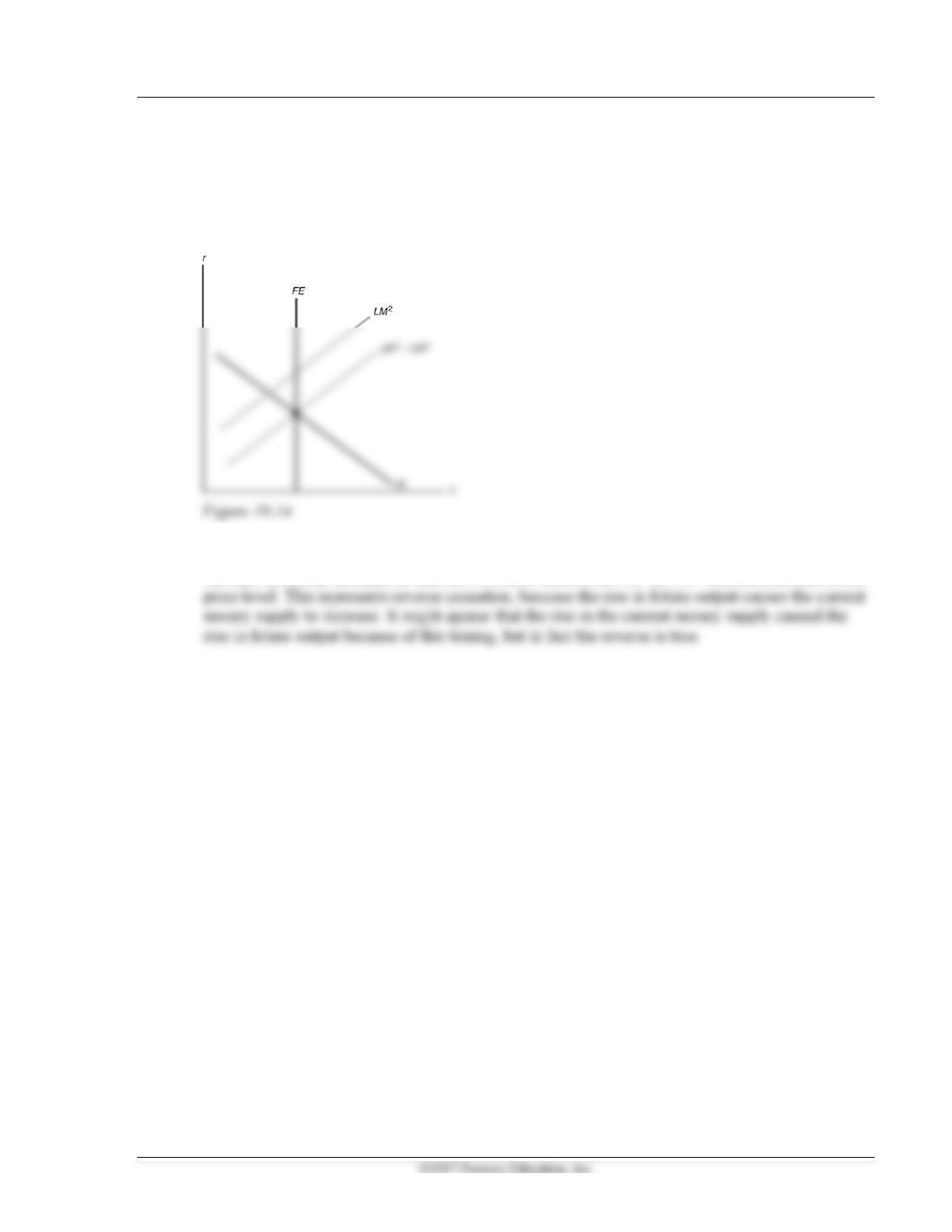
5. (a) An increase in expected future output increases money demand, so the LM curve shifts up and to
the left. As shown in Figure 10.14, the LM curve shifts from LM1 to LM2. General equilibrium in
the economy can be restored by shifting the LM curve from LM2 to LM3, which occurs as the
price level declines.
(b) If the Fed wants to stabilize the price level, then it increases the money supply in response to the
increase in money demand, so that the LM curve shifts from LM2 to LM3 without a decline in the

236 Abel/Bernanke/Croushore • Macroeconomics, Ninth Edition
Working with Macroeconomic Data
1. Generally, sharp changes up and down in productivity are correlated with business cycles.
Productivity often declines in recessions and rises faster in expansions.
2. a. Unanticipated money growth usually declines before recessions in the 1960s, 1970s, and 1980s.
3. The plots show that the forecasts are fairly rational, as they lie along a 45-degree line, as we would