Basic Econometrics, Gujarati and Porter
CHAPTER 10:
MULTICOLLINEARITY: WHAT HAPPENS IF THE REGRESSORS ARE
CORRELATED?
10.1 If X
k
is a perfect linear combination of the remaining explanatory
10.2 (a) No. Variable X
3i
is an exact linear combination of X
2i
, because
3 2
2 1.
i i
X X
= −
10.3 (a) Although the numerical values of the intercept and the slope
coefficients of PGNP and FLR have changed, their signs have not.
Also, these variables are still statistically significant. These changes
are due to the addition of the TFR variable, suggesting that there may
10.4 The relation may be rewritten as:
32
1 2 3 12.3 2 13.2 3
1 1
i i i i i
X X X X X
λ
λ
β β
λ λ
= − − = +
Therefore,
2 1
12.3 12.3 21.3
1 2
ˆ ˆ
( )( ) 1
r sqrt
λ λ
β β λ λ
= = − − = ±
10.5 (
a
) Yes. Economic time series data tend to move in the same
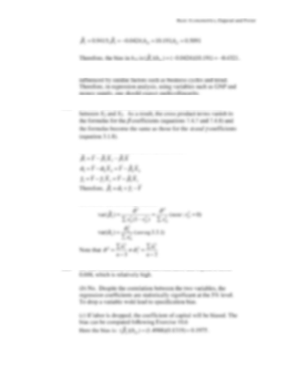
10.6 When wealth is removed from the model, the model is misspecified
and the income effect coefficient is biased. Hence, what one
observes in Eq. (10.6.4 ) is a biased estimate of the income
coefficient. The nature of the bias is as follows:
111
10.7 As discussed in Question 10.5, economic variables are often
10.8 (
a
) Yes. This is because the coefficient of correlation is zero
(
b
) It will be a combination, as shown below:
(c) No, for the following reasons:
10.9
(a) The correlation coefficient between labor and capital is about
112
will change the values of the other coefficients
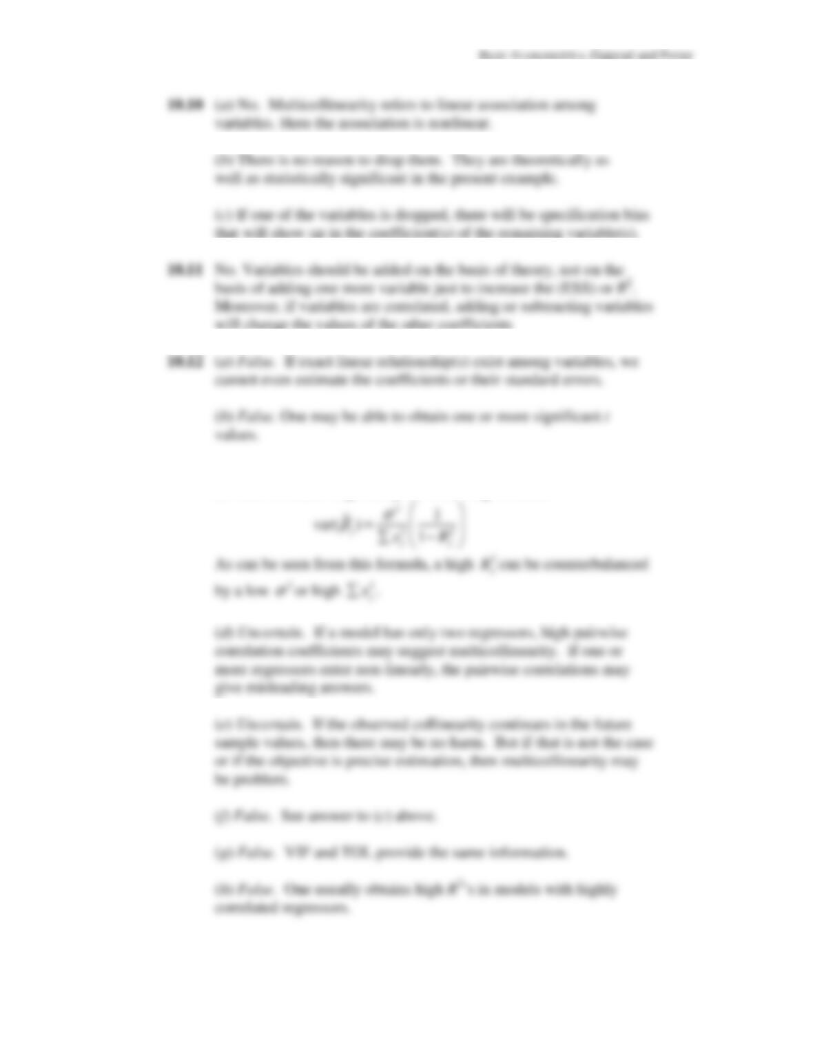
(c) False. As noted in the chapter (see Eq. 7.5.6), the variance of
an OLS estimator is given by the following formula:
Basic Econometrics, Gujarati and Porter
10.13 (a) Referring to Eq. (7.11.5), we see that if all the r
2
‘s are zero,
10.14 (a) Consider Eq. (7.11.5). If all the zero-order, or gross, correlations
10.15
(a) If there is perfect multicollinearity, (
X‘X
) becomes singular
10.16
(a) Since in the case of perfect multicollinearity the (
X’X
) matrix
Basic Econometrics, Gujarati and Porter
114
10.19
(a) Since the third regressor, (
1
t t
M M
−
−) is a linear combination of
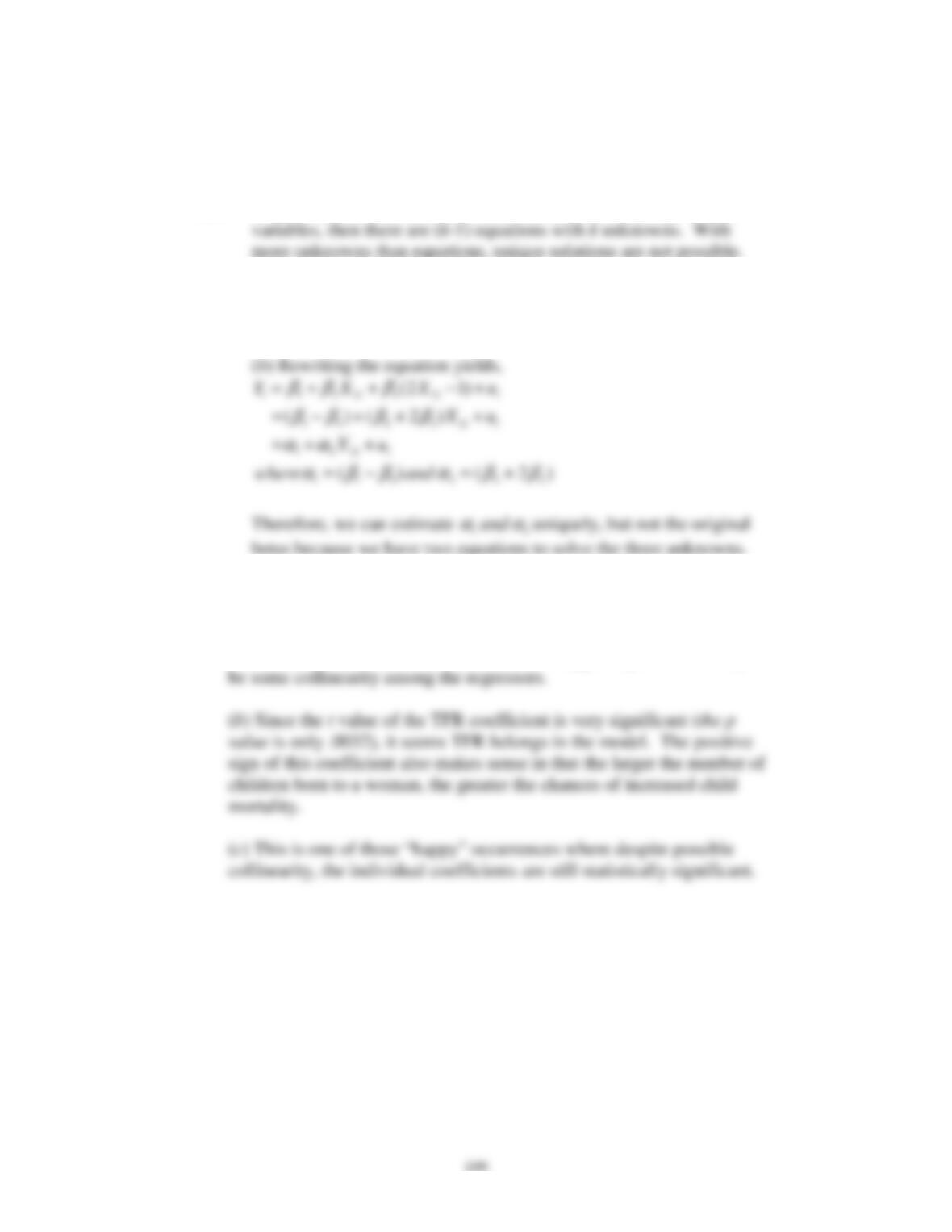
(b) If we re-specify the model as
10.20
Recall that
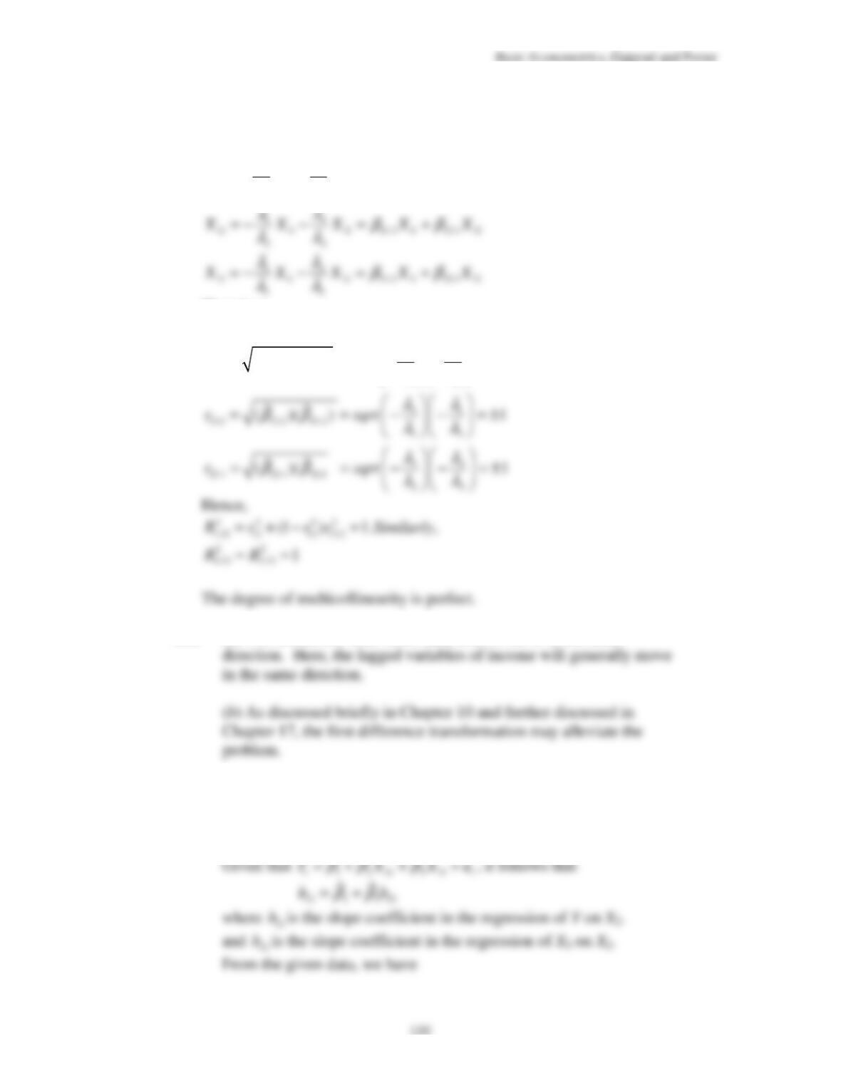
10.21
When there is perfect collinearity,
23
1
r
=
. Therefore, the
10.22
Recall that
ˆ ˆ ˆ ˆ ˆ ˆ
( ) [var( ) var( ) 2cov( , )]
se
β β β β β β
+ = + +
10.23
(a) Ceteris paribus, as
2
k
σ
increases, the variance of the estimated
Basic Econometrics, Gujarati and Porter
10.24
(a) Given the relatively high R
2
of 0.97, the significant F value and
(b) A priori, capital is expected to have positive impact on output. It
(c) It is a Cobb-Douglas type production function, as the given
(e) This equation implicitly assumes that there are constant returns
(g) As mentioned in (e), the author is trying to find out if there are
Basic Econometrics, Gujarati and Porter
116
Empirical Exercises
10.26
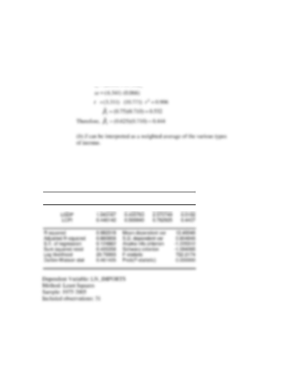
(a) The regression results of the modified model are:
ˆ
20.995 0.710
Y Z
= +
10.27
(a)
Dependent Variable: LIMPORTS
Method: Least Squares
Date: 11/11/00 Time: 10:16
Sample: 1970 1998
Included observations: 29
Variable Coefficient
Std. Error
t-Statistic
Prob.
C 1.975260
0.782070
2.525683
0.0180
Basic Econometrics, Gujarati and Porter
117
Variable Coefficient Std. Error t-Statistic Prob.
R-squared 0.992005 Mean dependent var 13.08472
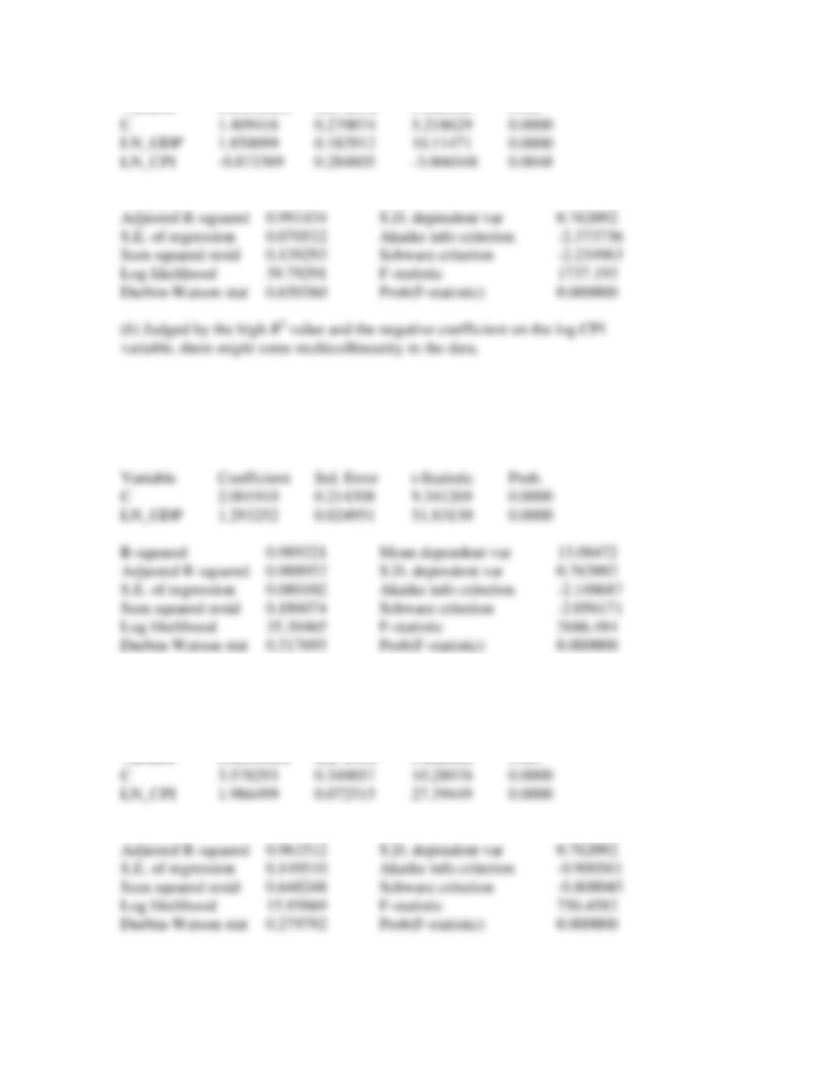
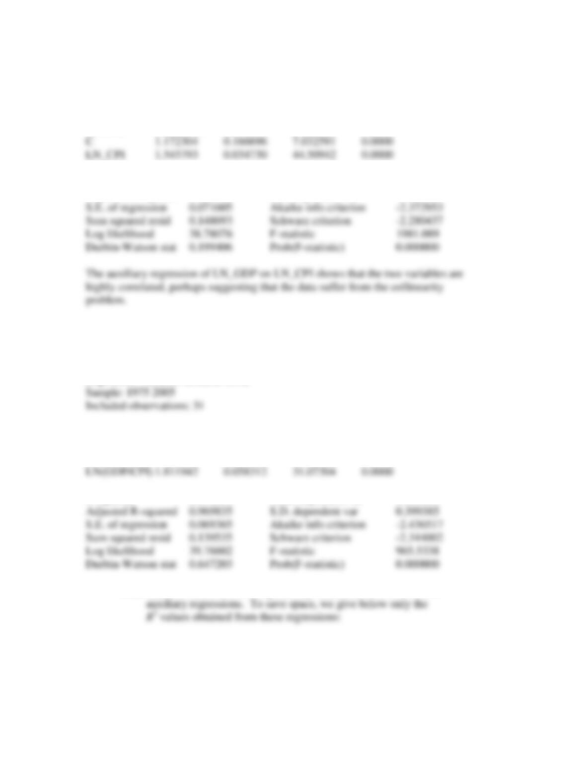
(c)
Dependent Variable: LN_IMPORTS
Sample: 1975 2005
Included observations: 31
Dependent Variable: LN_IMPORTS
Sample: 1975 2005
Included observations: 31
R-squared 0.962795 Mean dependent var 13.08472
Basic Econometrics, Gujarati and Porter
118
Dependent Variable: LN_GDP
Sample: 1975 2005
Included observations: 31
Variable Coefficient Std. Error t-Statistic Prob.
R-squared 0.985573 Mean dependent var 8.569723
Adjusted R-squared 0.985075 S.D. dependent var 0.586128
(d) The best solutions here would be to express imports and GDP in real terms by
dividing each by CPI (recall the ratio method discussed in the chapter). The results
are as follows:
Dependent Variable: LN(IMP/CPI)
Variable Coefficient Std. Error t-Statistic Prob.
C 1.442445 0.221017 6.526390 0.0000
R-squared 0.970841 Mean dependent var 8.299204
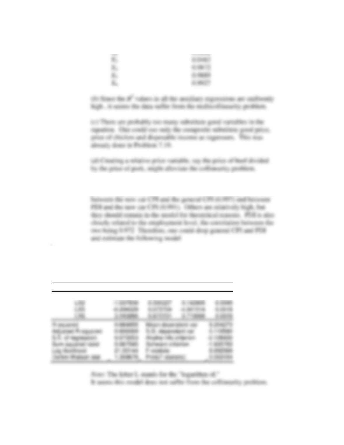
10.28
(a) Since there are five explanatory variables, there will be five
Basic Econometrics, Gujarati and Porter
119
Dependent Variable R
2
10.29
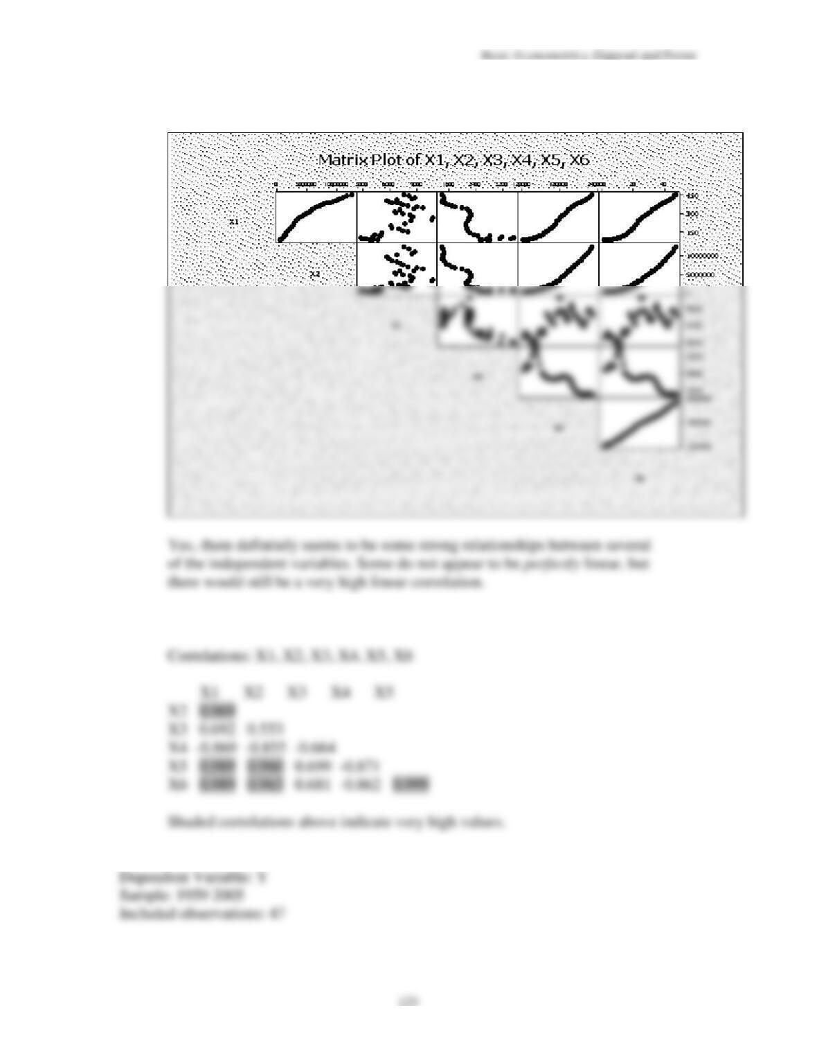
(a) and (c)Examining the correlation coefficients between the
possible explanatory variables, one observes a very high correlation
:
Dependent Variable: LY
Method: Least Squares
Sample: 1971 1986
Included observations: 16
Variable Coefficient
Std. Error
t-Statistic
Prob.
C -22.10374
8.373593
-2.639696
0.0216
(b) If we include all the X variables, we obtain the following results:
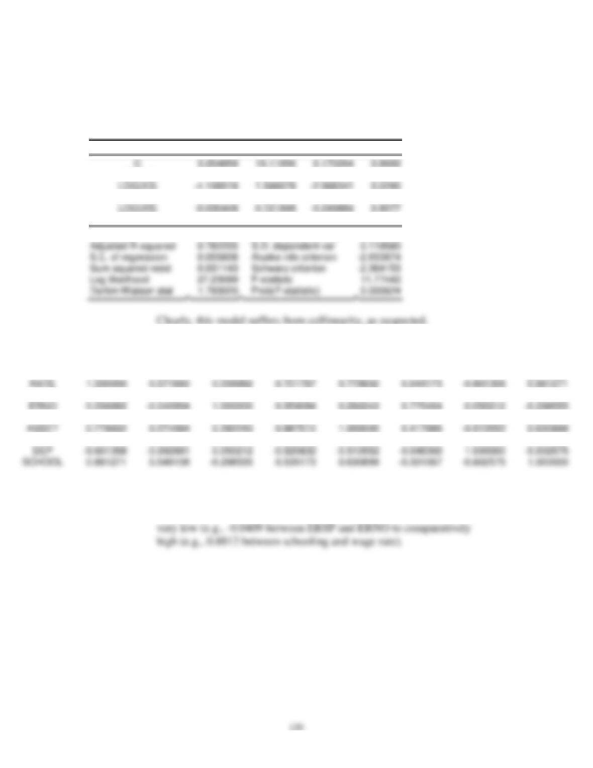
Basic Econometrics, Gujarati and Porter
Dependent Variable: LOG(Y)
Method: Least Squares
Sample: 1971 1986
Included observations: 16
Variable Coefficient
Std. Error
t-Statistic
Prob.
LOG(X2) 1.790153
0.873240
2.050012
0.0675
LOG(X4) 2.127199
1.257839
1.691154
0.1217
LOG(X6) 0.277792
2.036975
0.136375
0.8942
R-squared 0.854803
Mean dependent var 9.204273
10.30
First, we present the correlation matrix of the regressors:
RATE ERSP ERNO NEIN ASSET AGE DEP SCHOOL
ERSP 0.571693 1.000000 -0.040994 0.234426 0.274094 -0.015300 –0.692881 0.549108
NEIN 0.701787 0.234426 0.359094 1.000000 0.987510 0.502432 -0.520832 0.539173
AGE 0.044173 -0.015300 0.775494 0.502432 0.417086 1.000000 -0.048360 -0.331067
Note: Treat the last row in the preceding table as the last column
As this table shows, the pairwise, or gross, correlations range from
Basic Econometrics, Gujarati and Porter
121
(a)
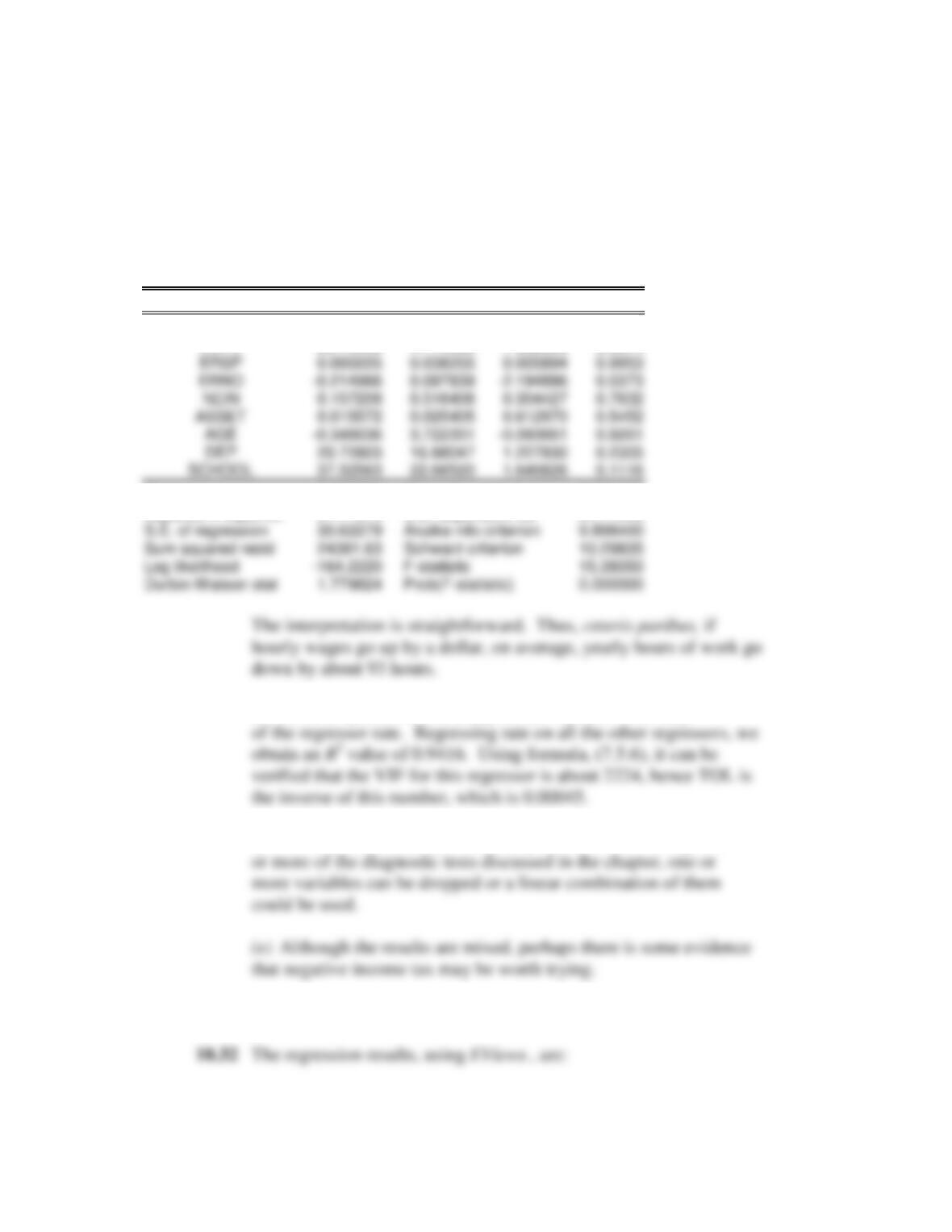
Regressing hours of work on all the regressors, we get the
following results:
Dependent Variable: HRS
Method: Least Squares
Sample: 1 35
Included observations: 35
Variable Coefficient
Std. Error
t-Statistic
Prob.
C 1904.578
251.9333
7.559849
0.0000
RATE -93.75255
47.14500
-1.988600
0.0574
R-squared 0.825555
Mean dependent var 2137.086
Adjusted R-squared 0.771879
S.D. dependent var 64.11542
(c)
To save space, we will compute the VIF and TOL only
(d)
Not all the variables are necessary in the model. Using one
10.31
This is for a class project.
Basic Econometrics, Gujarati and Porter
122
Dependent Variable: Y
Method: Least Squares
Sample: 1947 1961
Included observations: 15
Variable Coefficient Std. Error t-Statistic Prob.
C -3017441. 939728.1 -3.210973 0.0124
X1 –20.51082 87.09740 -0.235493 0.8197
R-squared 0.9955 Adjusted R-squared 0.9921
S.E. of regression 295.6219
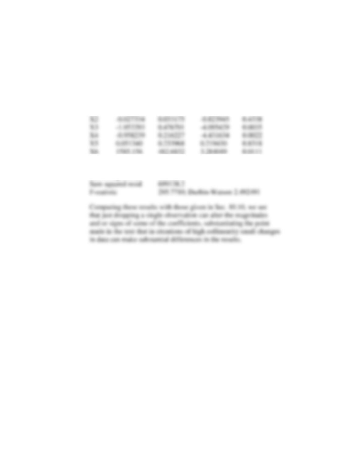
10.33
(a)
(b)
The correlation matrix for the independent variables is:
(c) and (d)
Basic Econometrics, Gujarati and Porter
Variable Coefficient Std. Error t-Statistic Prob.
C -11304.74 9963.786 -1.134583 0.2633
X1 87.45286 6.649853 13.15110 0.0000
R-squared 0.999398 Mean dependent var 101822.8
10.34
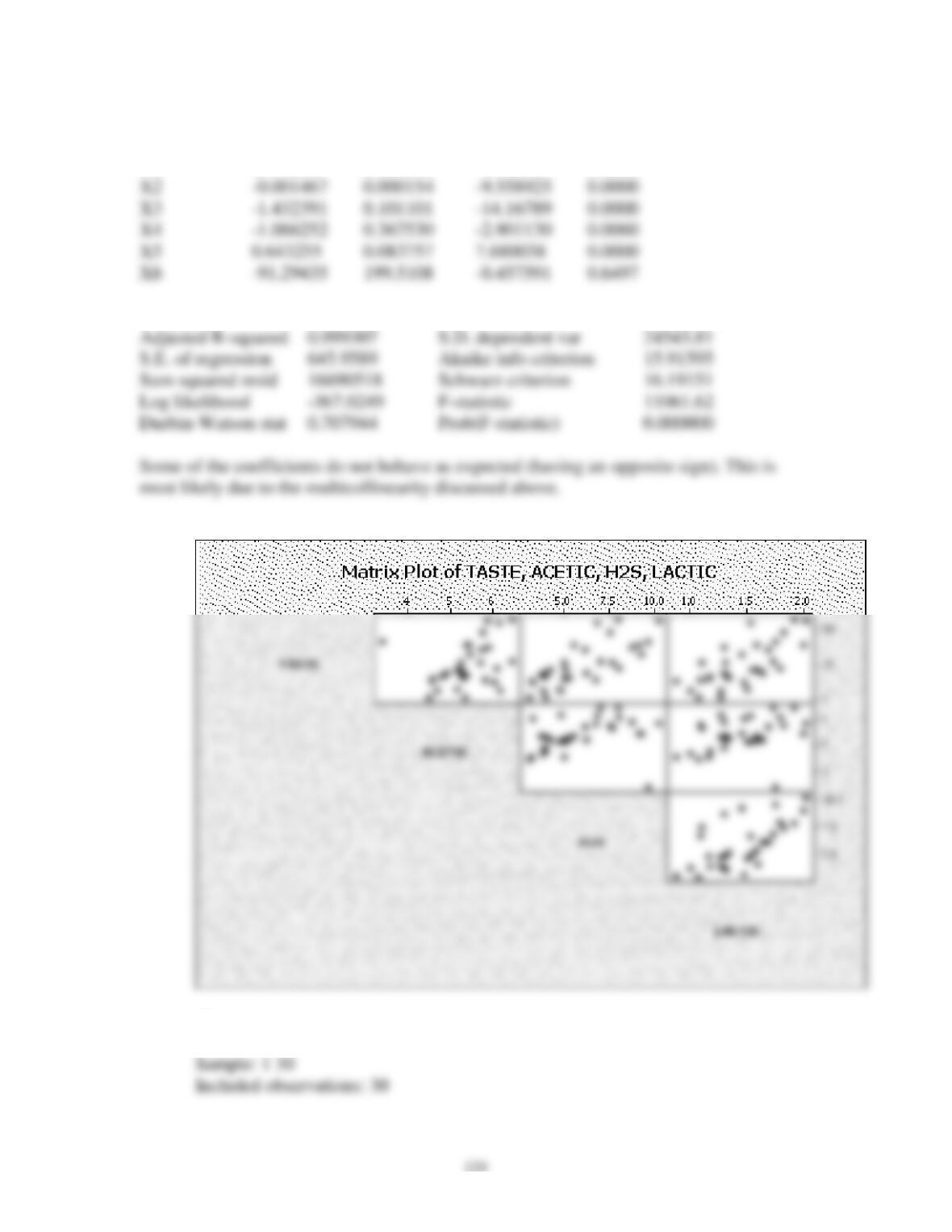
(a)
(b)
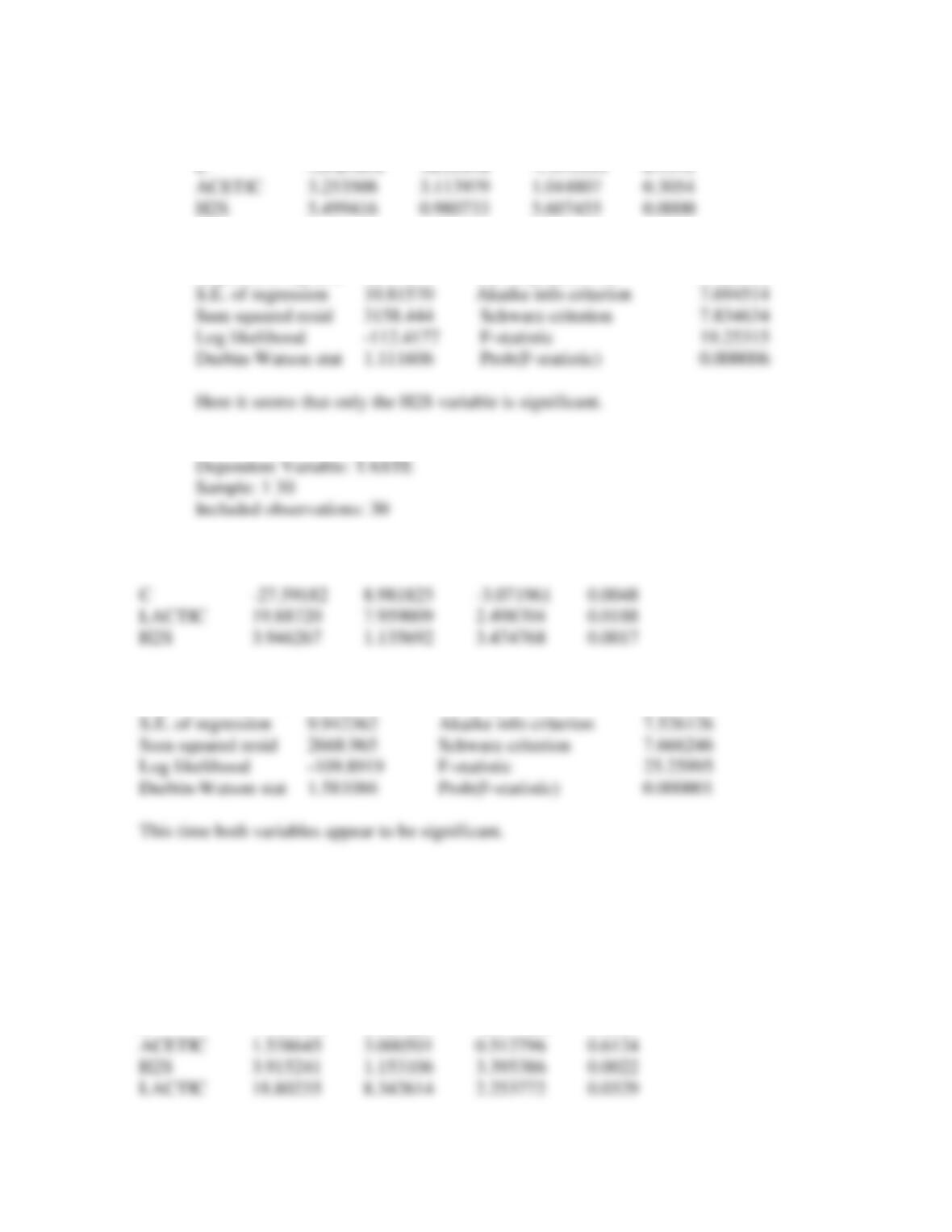
Dependent Variable: TASTE
Basic Econometrics, Gujarati and Porter
125
Variable Coefficient Std. Error t-Statistic Prob.
R-squared 0.587826 Mean dependent var 24.53333
Adjusted R-squared 0.557294 S.D. dependent var 16.25538
(c)
Variable Coefficient Std. Error t-Statistic Prob.
R-squared 0.651702 Mean dependent var 24.53333
Adjusted R-squared 0.625903 S.D. dependent var 16.25538
(d)
Dependent Variable: TASTE
Sample: 1 30
Included observations: 30
Variable Coefficient Std. Error t-Statistic Prob.
C -34.13491 15.67628 -2.177488 0.0387
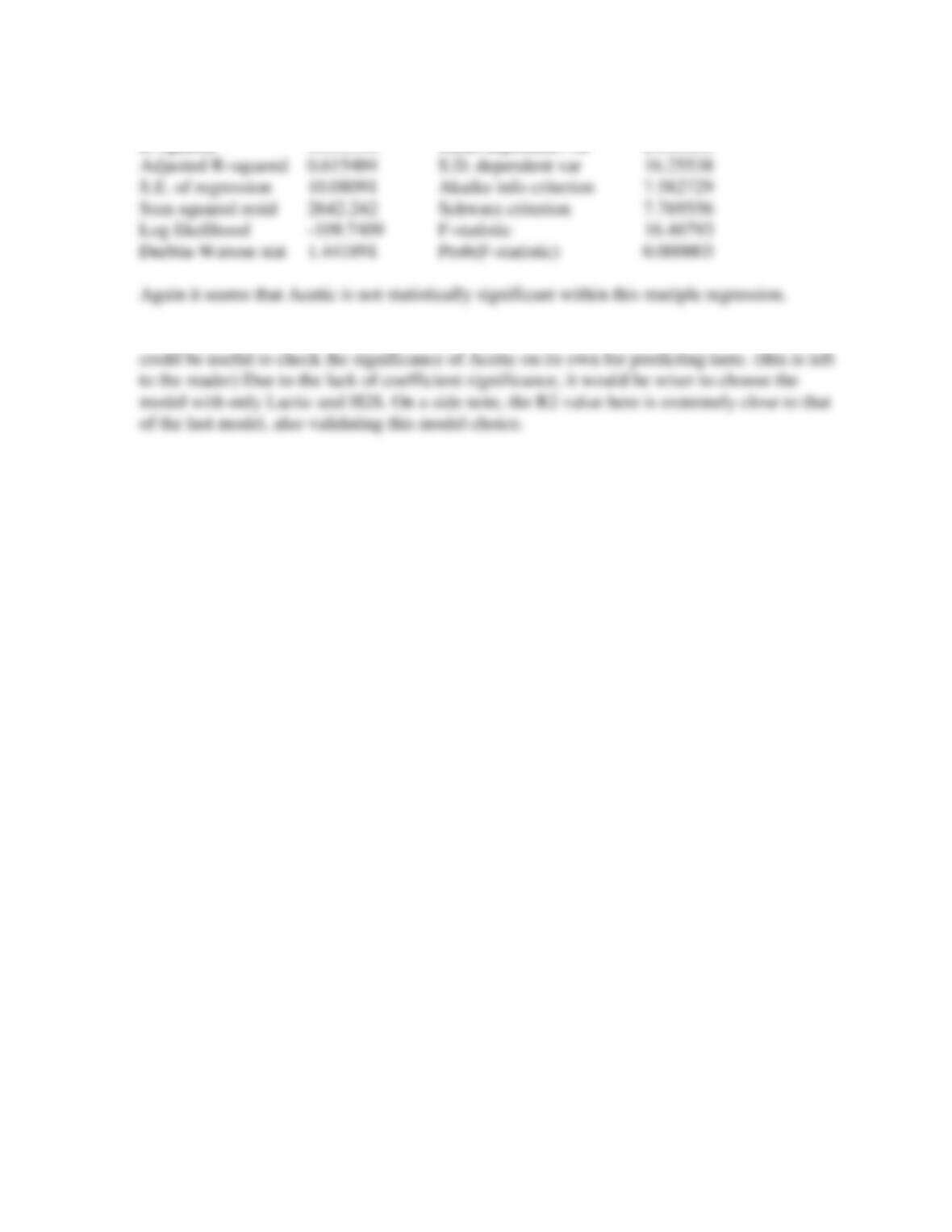
Basic Econometrics, Gujarati and Porter
126
R-squared 0.655190 Mean dependent var 24.53333
(e) and (f) It very well may be that the Acetic variable is highly linearly related to H2S. It