233
CHAPTER 10
Introduction to Economic
Fluctuations
Notes to the Instructor
Chapter Summary
This chapter introduces students to short–run economic fluctuations, the importance of sticky prices, and
the aggregate demand–aggregate supply model. The main aims of the chapter are the following:
2. To introduce a simple quantity–equation aggregate demand curve (prior to the more general IS–LM
theory of aggregate demand that is presented in Chapters 11 and 12).
4. To introduce the idea of shocks to aggregate demand and aggregate supply as a source of economic
fluctuations.
Comments
This is obviously a good point at which to review the models of the long run presented in Part II of the
textbook and to explain why these are not adequate for understanding the short–run behavior of the
economy. (Supplement 10–8 may be helpful for this.) Part IV of the book will present the students with
many new models at a fast rate, so it is important that they have a good grasp of the long–run models of
Part II. It also is helpful to emphasize that short–run models are a supplement, not an alternative, to long–
run models. All the time that students are studying the short run, they should try to retain the long–run
Use of the Web Site
Since this is the point in the course at which business cycles come to the forefront, it is a natural time to
make much use of the Data Plotter. The plotter can be used in particular to show the irregular fluctuations
in GDP that have to be explained and also to demonstrate other basic stylized facts.
Use of the Dismal Scientist Web Site
234 | CHAPTER 10 Introduction to Economic Fluctuations
Chapter Supplements
This chapter includes the following supplements:
10-1 The Dating of Business Cycles
10-3 Are Prices Sticky? I: Evidence from Individual Transactions (Case Study)
10-4 Are Prices Sticky? II: Mail–Order Evidence (Case Study)
10-5 Price Stickiness and Pareto Efficiency
10-7 Understanding Business Cycles II: Modeling Cycles
10-9 The Cost of Business Cycles
10–10 Additional Readings
!Figure 10-2
Lecture Notes | 235
Lecture Notes
Introduction
The classical model developed in Part II of the book explains the behavior of key
macroeconomic variables in the long run. But the task of macroeconomics goes beyond this.
Macroeconomists and policymakers are also concerned with the year-to–year and quarter–to–
quarter fluctuations of the economy. Real GDP does not grow smoothly through time, as the
Solow growth model might suggest; rather it sometimes grows very rapidly, sometimes less
10-1 The Facts about the Business Cycle
GDP and Its Components
The growth rate of real GDP has fluctuated considerably over time and occasionally is negative
during periods of recession. In the United States, the National Bureau of Economic Research is
the official arbiter of when recessions begin and end. The NBER considers various economic
indicators in making its determination about business cycle turning points and does not follow
the conventional rule of thumb that defines a recession as two successive quarters of negative
Unemployment and Okun’s Law
The economist Arthur Okun noted that we should expect to find a relationship between
unemployment and real GDP. When the unemployment rate is higher, we should presumably
expect to find that real GDP is lower. He suggested a rule of thumb, which has become known as
Okun’s law:
Leading Economic Indicators
Economists often need to develop forecasts of where the economy is heading in the future. One
approach is to consider so–called leading indicators, which are economic variables that typically
fluctuate in advance of overall economic activity. For the United States, the Conference Board, a
private business research group, constructs the Index of Leading Economic Indicators each
month. The index is composed of ten data series that are believed to anticipate changes in
economic activity roughly six to nine months in advance. The index includes the following:
2. Average weekly initial claims for unemployment insurance
!Supplement 10–1,
“The Dating of
Business Cycles”
!Figure 10-1
!Supplement 1–3,
“When Is the
Economy in a
!Figure 10-3
!Figure 10-4
4. Manufacturer’s new orders for nondefense capital goods, excluding aircraft
6. Building permits for new private housing units
8. Leading Credit Index
10. Average consumer expectations for business and economic conditions
10-2 Time Horizons in Macroeconomics
How the Short Run and Long Run Differ
The models covered in the text apply to either the short run, the long run, or the very long run.
These designations have more to do with the flexibility or inflexibility of factors of production
prices than with strict time limits, as shown in the table below.
Model
Assumptions
Time Frame
Short run
Sticky prices, possible
unemployment of labor and
capital
Month–to–month or year–
to–year
Long run
Flexible prices, full employment
of labor and capital; constant
capital, labor force, and
technology
Several years
Very long run
Flexible prices, full employment
of labor and capital; variable
capital, labor force, and
technology
Several decades
Case Study: If You Want to Know Why Firms Have
Sticky Prices, Ask Them
Alan Blinder studied the reasons for price stickiness by going directly to the source—the firms.
Blinder asked managers how often they changed prices—most often, the answer was once or
twice a year—and found clear evidence of price stickiness. Next, Blinder presented the
The Model of Aggregate Supply and Aggregate Demand
The implications of sticky prices are far–reaching. The most important point is that, when prices
are sticky, GDP need not always be at its natural rate. Further, monetary and fiscal policies can
!Table 10-1
!Table 10-2
!Supplement 10–3,
“Are Prices
Sticky? I:
Evidence from
Order Evidence
10–3 Aggregate Demand
The Quantity Equation as Aggregate Demand
Aggregate demand gives a relationship between the price level and the quantity of goods and
services demanded. Like a regular demand curve, it slopes downward: At a higher price level,
fewer goods are demanded. The reasons that aggregate demand slopes downward are more
complex than this analogy suggests. We defer the detailed theory of aggregate demand to
Chapters 11 and 12 and work for the present with the simplest possible aggregate demand curve,
which is based on the quantity equation. Recall that
Why the Aggregate Demand Curve Slopes Downward
This equation implies a negative relationship between Y and P. If income is higher, there is a
greater demand for real money balances. If the money supply is fixed in nominal terms, then
Shifts in the Aggregate Demand Curve
Since the aggregate demand curve is drawn on a diagram with P and Y on the axes, it will shift if
either of the two other variables (M and V) changes. If the money supply is reduced, holding V
fixed, then real balances are lower and so output must be lower. The aggregate demand curve
shifts in. The opposite is true if M is increased. Similarly, a decrease in velocity will shift the
aggregate demand curve in; an increase will shift it out.
10–4 Aggregate Supply
The Long Run: The Vertical Aggregate Supply Curve
We know that the supply of goods and services in the long run depends upon the technology and
the available stocks of capital and labor. We also know that the long–run analysis is conducted
entirely in real terms. In other words, the supply of goods and services in the long run does not
depend upon the price level in the economy. This means that the long–run aggregate supply
curve (LRAS) is vertical at Y.
Economic growth, in this setting, is captured by the fact that the LRAS curve shifts to the
right over time. As the technology improves or the economy gets more capital and labor, more
!Figure 10-5
!Figure 10-6
!Figure 10-7
!Figure 10–10
238 | CHAPTER 10 Introduction to Economic Fluctuations
We can now see why this model, while adequate for the long run, is not of much use for
explaining short–run fluctuation. No matter how much the aggregate demand curve moves
around, we can see from this model that the only long–run consequence will be movements in
the price level. The classical dichotomy holds in the long run. If prices were flexible in the short
run as well as the long run, the classical dichotomy would hold in the short run, and changes in
aggregate demand would have no effect on output.
The Short Run: The Horizontal Aggregate Supply Curve
There is a very simple way to capture the idea of price stickiness in our model. Suppose that in
the short run (perhaps a period of three months or so), the price level does not change at all.
Then we can represent this by a short–run aggregate supply curve that is horizontal.
A story to demonstrate this is as follows. Consider a representative firm in the economy.
Once every three months, all the vice presidents meet with the chief executive officer. The vice
president of finance comes in with his Excel spreadsheet and presents a picture of the financial
side; the vice president of production comes in with his spreadsheet and explains the current cost
side; the vice president of marketing comes in with his spreadsheet and gives his forecasts for
demand over the next few months. The CEO listens to them all. After carefully weighing all
their arguments, she decides on the price that the firm will charge for its product. For the next
three months, they then sell as much or as little as is demanded at that price. After three months,
they go through this process again.
From the Short Run to the Long Run
What does the adjustment to the long run look like? Following a negative aggregate demand
shock, firms face lower demand and so reduce output at the fixed price level. If the economy
was originally at the natural rate, then it goes into recession. Given the fall in demand, prices and
wages will start to fall and output will increase. The economy moves back down the aggregate
demand curve to the new long–run equilibrium. The recovery from a recession is characterized
by falling prices.
Case Study: A Monetary Lesson from French History
An example of how a monetary contraction affects the economy comes from eighteenth–century
France. At that time, the monetary value of each coin was set by government decree. On
September 22, 1724, the government reduced the value of its currency by 20 percent overnight.
During the next seven months, the value of the money stock was reduced further for a total
decline of 45 percent. The government sought this change to lower prices to a level it deemed
acceptable. Although wages and prices fell, they did not decline by the full 45 percent. And it
!Figure 10-8
!Figure 10-9
!Figure 10–11
!Figure 10–12
Lecture Notes | 239
FYI: David Hume on the Real Effects of Money
The work of eighteenth–century philosopher and economist David Hume was highlighted in
Chapter 5 as a foundation for the quantity theory of money and the analysis of how growth in the
money supply eventually leads to higher inflation. Hume also was aware, however, that in the
short run, changes in the money supply have real effects on the economy. Perhaps his writing on
this topic was informed by knowledge of the French experience described in the case study.
Shocks to Aggregate Demand
When prices are sticky, exogenous shocks to aggregate demand will cause output fluctuations.
The associated cyclical fluctuations are usually thought to be costly and undesirable. Since the
monetary authorities can affect the level of demand by changing the money supply, it is natural
Shocks to Aggregate Supply
Shocks to the economy need not always affect aggregate demand; they might affect aggregate
supply. Such shocks affect firms’ costs and hence the prices that they charge; thus they are
sometimes called price shocks. Examples include agricultural shocks, such as bad weather,
which raises food prices; government regulation of industry; increased union power, which
increases wages; and increases in world energy prices. All of these shocks have the effect of
increasing the general price level. If aggregate demand is unchanged, then output will fall.
Case Study: How OPEC Helped Cause Stagflation in the 1970s
and Euphoria in the 1980s
Supply shocks significantly affected the world’s economies in the 1970s. The Organization of
Petroleum Exporting Countries (OPEC) colluded to reduce the supply of oil and raise its price.
There were major oil price rises in 1974 and at the end of the decade. This led to stagflation (that
is, stagnation, or recession, combined with inflation) in many countries. In the 1980s, oil prices
!Supplement 10–5,
!Figure 10–14
10–6 Conclusion
We now have a basic model of the economy in the short and long run. Price adjustment tends to
return the economy to the natural rate of output in the long run. The natural rate of output grows
!Supplement 10–8,
“The Economy in
ADDITIONAL CASE STUDY
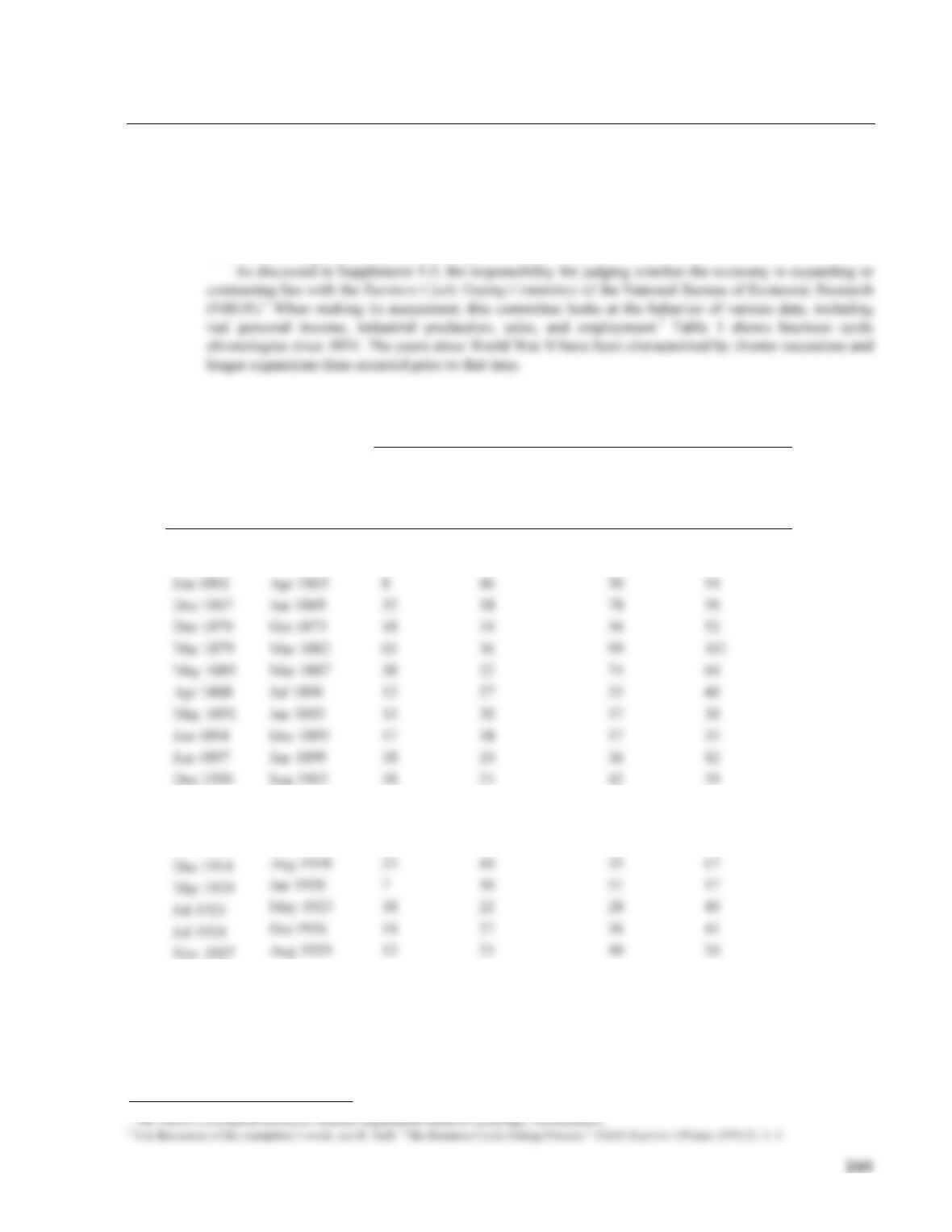
10–1 The Dating of Business Cycles
Economies exhibit short–run fluctuations in output and other variables, known as the business cycle. When
the economy is doing well, so that output and employment are rising, it is said to be expanding. If output
and employment start to fall, the economy is said to be contracting (or in recession). The turning point
from expansion to contraction is known as the peak of the business cycle, while the turning point from
contraction to expansion is called the trough.
Table 1 Business Cycle Expansions and Contractions
Duration in Months
Duration in Months
Trough
Peak
Contraction
Expansion
Trough
From
Previous
Trough
Peak From
Previous
Peak
Dec 1854
Jun 1857
30
Dec 1858
Oct 1860
18
22
48
40
Jun 1861
Apr 1865
46
30
54
Dec 1867
Jun 1869
32
18
78
50
Dec 1870
Oct 1873
18
34
36
52
Mar 1879
Mar 1882
65
36
99
101
May 1885
Mar 1887
38
22
74
60
Apr 1888
Jul 1890
13
27
35
40
May 1891
Jan 1893
10
20
37
30
Jun 1894
Dec 1895
17
18
37
35
Jun 1897
Jun 1899
18
24
36
42
18
21
42
39
Aug 1904
May 1907
23
33
44
56
Jun 1908
Jan 1910
13
19
46
32
Jan 1912
Jan 1912
24
12
43
36
Dec 1914
23
44
35
67
Mar 1919
Jan 1920
10
51
17
Jul 1921
May 1923
18
22
28
40
Jul 1924
14
27
36
41
Nov 1927
13
21
40
34
Mar 1933
May 1937
43
50
64
93
Jun 1938
Feb 1945
13
80
63
93
1 The NBER is a nonprofit economic research organization based in Cambridge, Massachusetts.
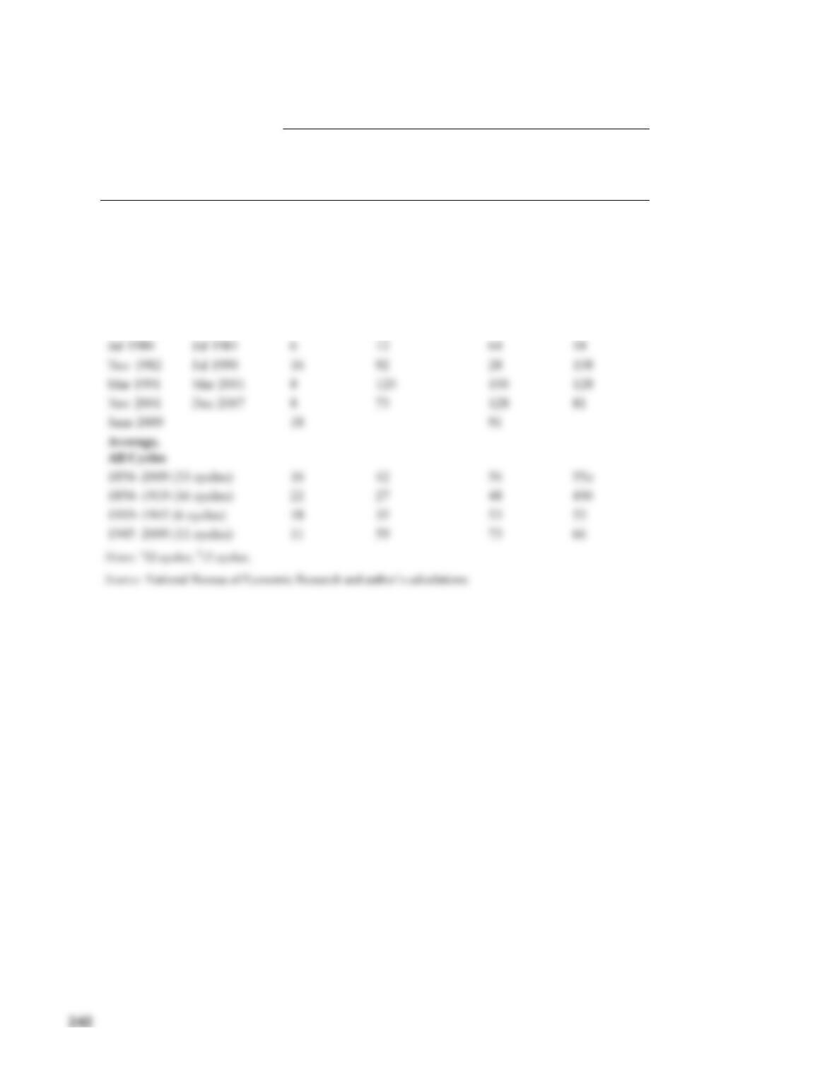
Table 1 (Continued)
Duration in Months
Duration in Months
Trough
Peak
Contraction
Expansion
Trough
From
Previous
Trough
Peak From
Previous
Peak
Oct 1945
Nov 1948
8
37
88
45
Oct 1949
Jul 1953
11
45
48
56
May 1954
Aug 1957
10
39
55
49
Apr 1958
Apr 1960
8
24
47
32
Jan 1961
Dec 1969
10
106
34
116
Nov 1970
Nov 1973
11
36
117
47
Mar 1975
Jan 1980
16
58
52
74
Jul 1980
Jul 1981
12
64
18
Nov 1982
Jul 1990
16
92
28
108
Mar 1991
Mar 2001
8
120
100
128
Nov 2001
Dec 2007
73
128
81
June 2009
18
91
1854–2009 (33 cycles)
16
42
56
55a
1854–1919 (16 cycles)
22
27
48
49b
1919–1945 (6 cycles)
18
35
53
53
1945–2009 (11 cycles)
11
59
73
66
ADDITIONAL CASE STUDY
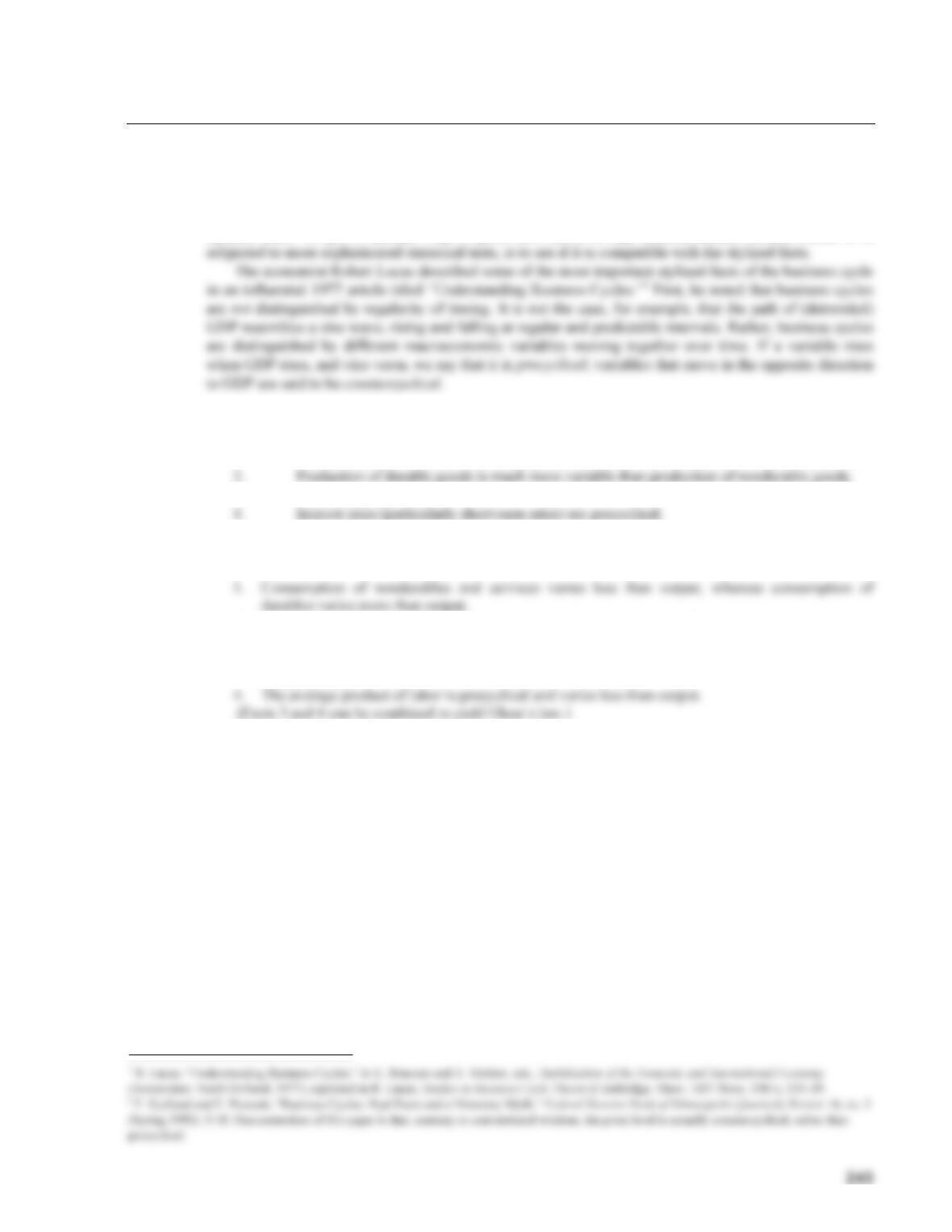
10–2 Understanding Business Cycles I: The Stylized Facts
A major task of macroeconomics is to explain the business cycle, which is a shorthand term for some
statistical regularities, or stylized facts, in economic data. Stylized facts are a compact way of describing
the main features of macroeconomic data. Macroeconomics involves building models that can explain the
stylized facts. To put it another way, a good first check of any macroeconomic model, before it is
Among the principal stylized facts noted by Lucas were the following:
1. Output movements tend to be correlated across sectors of the economy. It is not the case that
the business cycle is an accidental by–product of unconnected cycles in different industries.
3. Prices are procyclical.
5. Nominal money is procyclical.
Other stylized facts of the business cycle include the following:
2. Investment, and more particularly inventory investment, varies more than output.
3. Hours worked are procyclical and vary about as much as output. Part of this variation is the result
of variation in employment and part is the result of variation in hours per worker, both of which
are procyclical.
5. Real wages are slightly procyclical.
A detailed discussion of many of these stylized facts can also be found in a paper by Finn Kydland
and Edward Prescott.2