Chapter 10
Systems of Equations
◼ Exercises
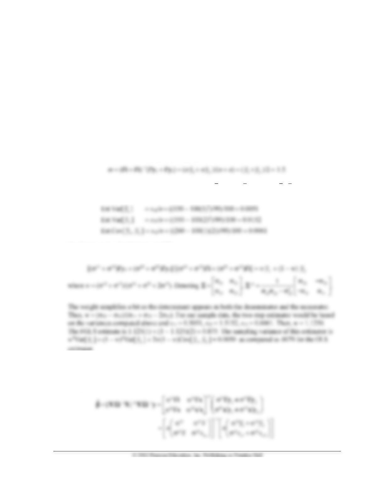
1. The model can be written as
11
22
.
=+
yi
yi
Therefore, the OLS estimator is
The sampling variance would be Var[m] = (1/2)2{Var[
1
y
] + Var[
2
y
] + 2Cov[(
1,y
2
y
)]}.
We would estimate the parts with
Combining terms, Est.Var[m] = 0.0079.
The GLS estimator would be
estimator.
2. The model is y =
1
2
y
y
= X + =
11
22
+
i0
0x
, 2 =
II
II
11 12
12 22
.
The generalized least squares estimator is
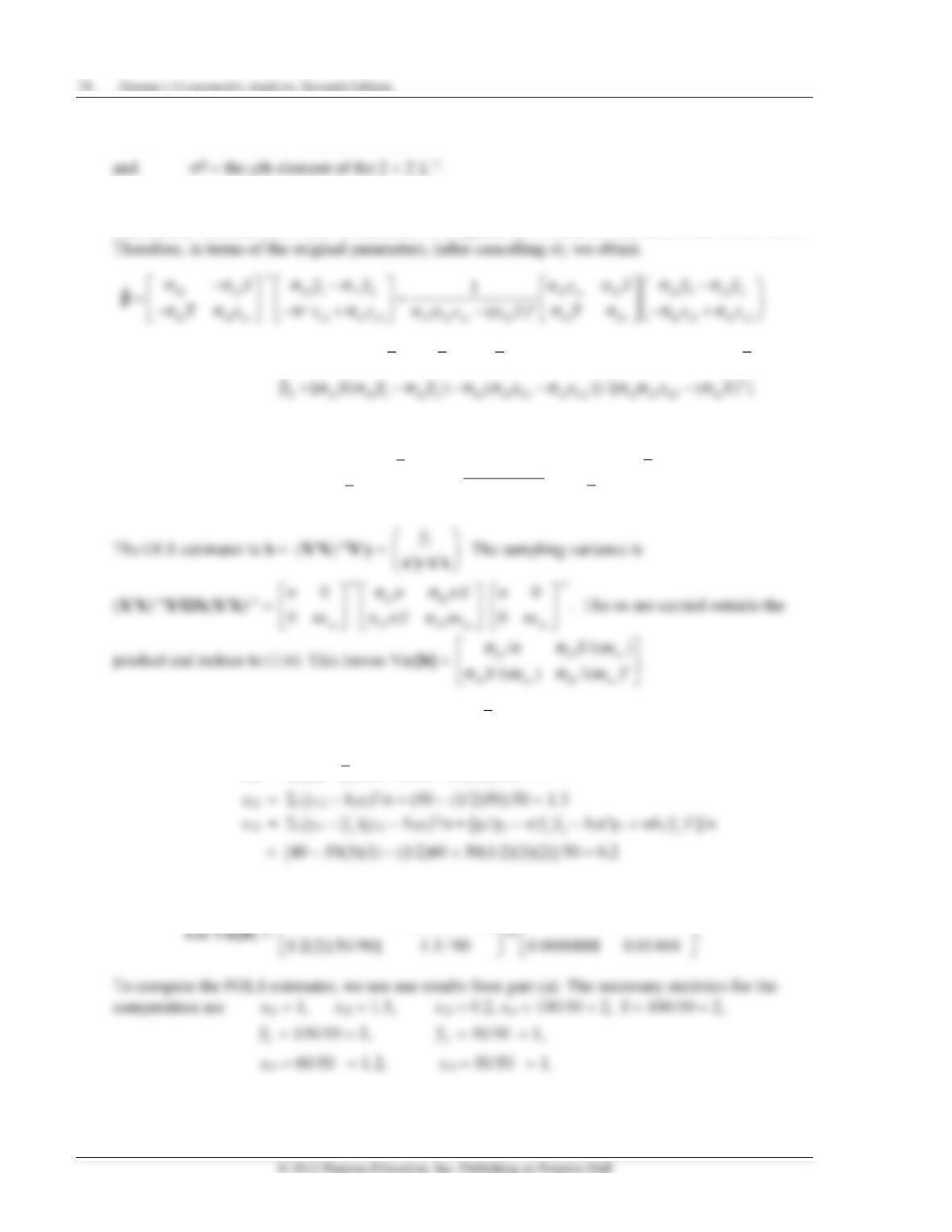
where sxx = xx/n, sx1 = xy1/n, sx2 = xy2/n
To obtain the explicit form, note, first, that all terms ij are of the form
2
11 22 12
/( ).
ji
−
But, the
denominator in these ratios will be cancelled as it appears in both the inverse matrix and in the vector.
The two elements are
2
1 11 22 1 12 2 12 12 1 11 2 11 22 12
ˆ[ ( ) ( )] / [ ( ) ]
XX X X XX
s y y x s s s x
= − − − −
The asymptotic covariance matrix is
[X−1X]−1 =
11
11 12
22 12
12 22 2
12 11
11 22 12
.
xx
xx
x
xn
nxs
xs
−−
−
=
−
−
Using the results above, the OLS coefficients are b1 =
1
y
= 150/50 = 3 and b2 = xy2/xx = 50/100 =
1/2. The estimators of the disturbance (co-)variances are
s11 = i (yi1 −
1
y
)2/n = (500 − 50(3)2)/50 = 1
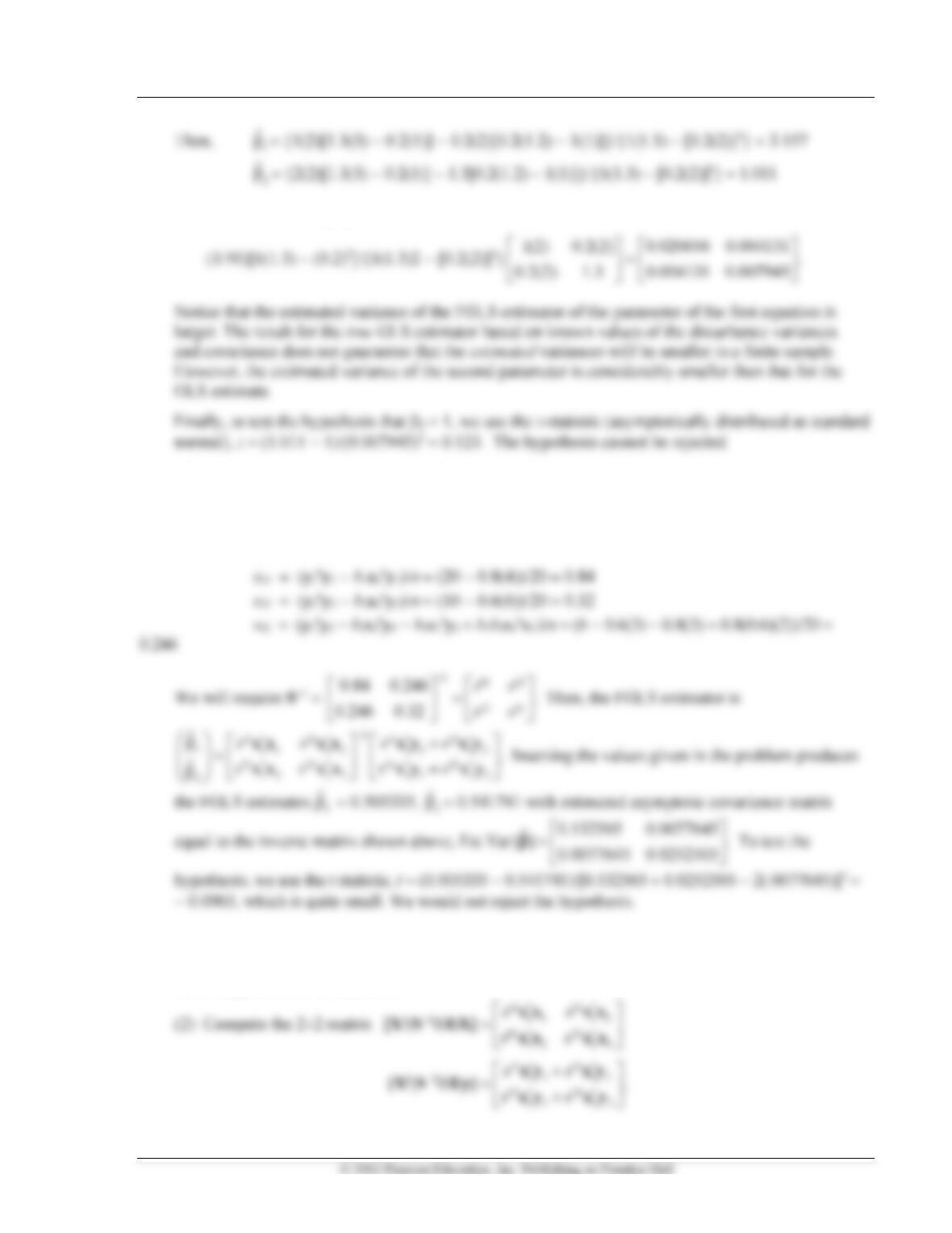
Therefore, we estimate the asymptotic covariance matrix of the OLS estimates as
1/50 0.2(2)[50(90)] 0.02 0.0000888 .
Chapter 10 Systems of Equations 75
The estimate of the asymptotic covariance matrix is
3. The ordinary least squares estimates of the parameters are
b1 = x1y1/x1x1 = 4/5 = 0.8 and b2 = x2y2/x2x2 = 6/10 = 0.6.
Then, the variances and covariance of the disturbances are
To compute the maximum likelihood estimates, we would begin with the OLS estimates of 11, 22,
and 12. Then, we iterate between the following calculations
(1) Compute the 2 2 matrix, S−1.

Chapter 10 Systems of Equations 77
Compare this estimate to the previous one. If they are similar enough, exit the iterations.
(5) Go back to step (1) and continue.
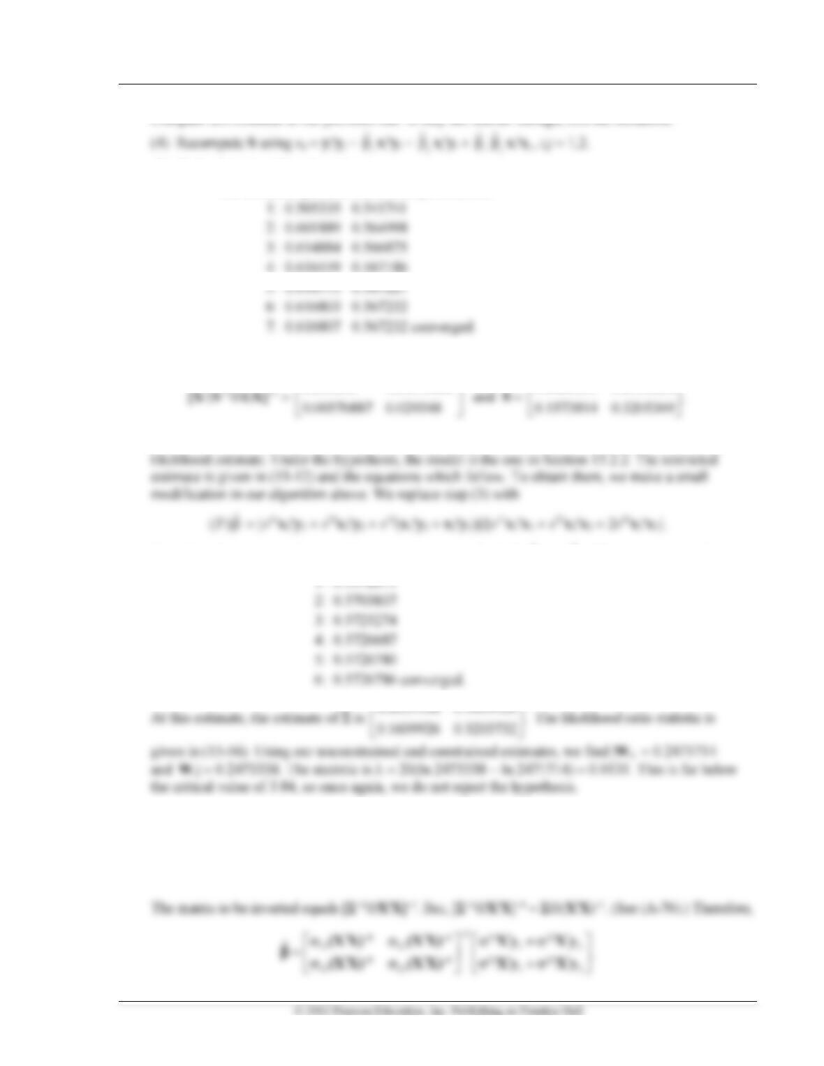
Our iterations produce the two slope estimates
At convergence, we find the estimate of the asymptotic covariance matrix of the estimates as
0.155355 0.00576887
0.8483899 0.1573814 .
To use the likelihood ratio method to test the hypothesis, we will require the restricted maximum
Step (4) is then computed using this common estimate for both
1
ˆ
and
2
ˆ.
The iterations produce
4. The GLS estimator is
111 12
11 12
12
12 22
12 22
12
ˆ.
−
+
=
+
X y X y
X X X X
X y X y
X X X X
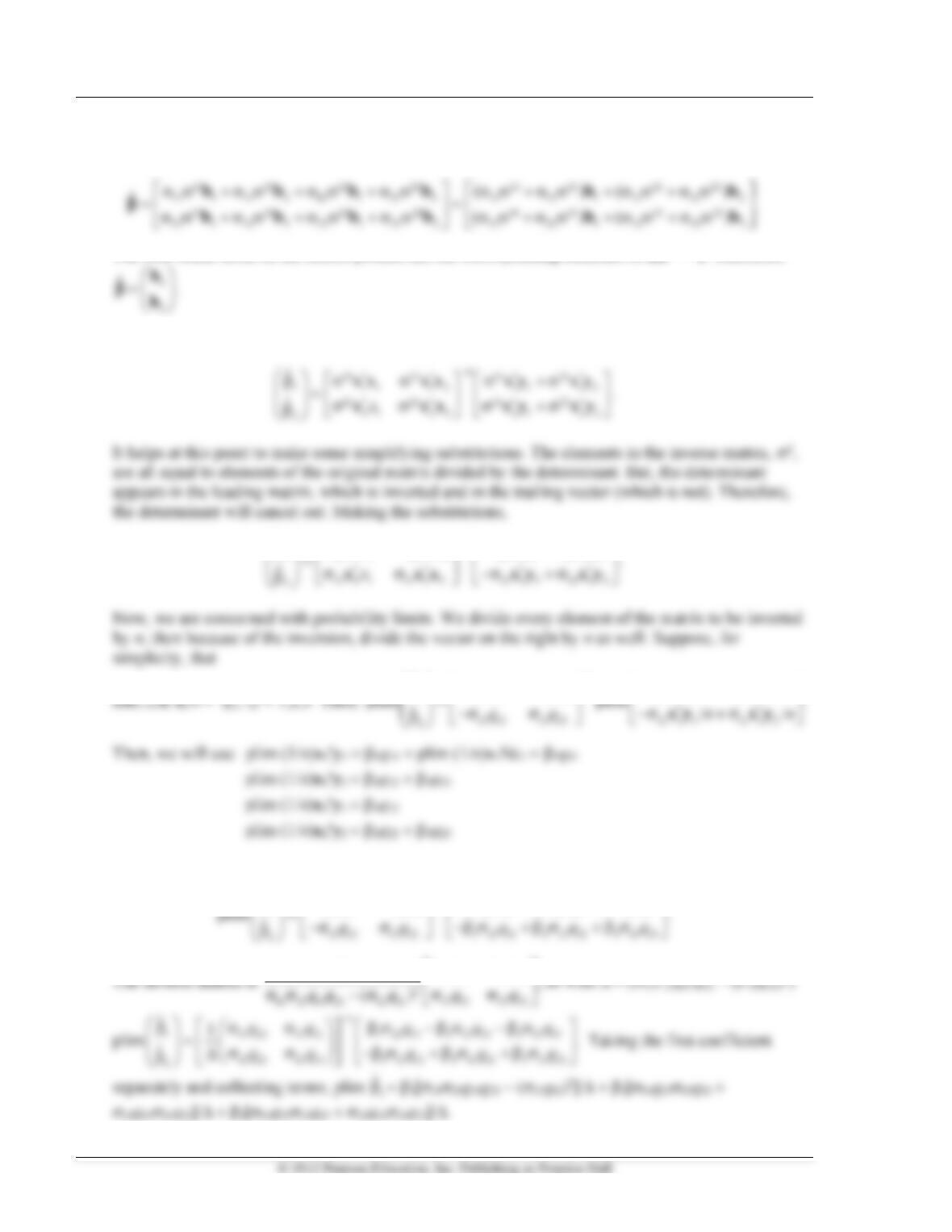
78 Greene • Econometric Analysis, Seventh Edition
We now make the replacements Xy1 = (XX)b1 and Xy2 = (XX)b2. After multiplying out the
product, we find that
The four scalar terms in the matrix product are the corresponding elements of −1 = I. Therefore,
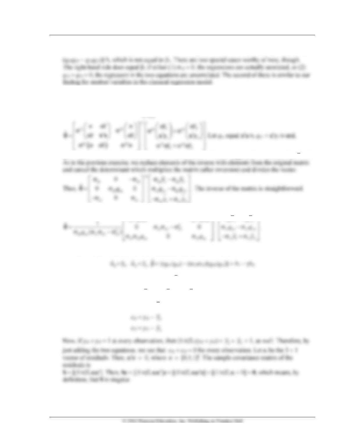
5. The algebraic result is a little tedious, but straightforward. The GLS estimator which is computed is
1
1 22 1 1 12 1 2 22 1 1 12 1 2
ˆ
−
− −
x x x x x y x y
1
1 22 11 12 12 22 1 1 12 1 2
ˆ//
q q n n
−
− −
x y x y
Therefore, after multiplying out all the terms,
1
1 22 11 2 12 12 3 12 13
1 22 11 12 12
ˆ
q q q
qq
−
− −
−
11 22 12 12
1,
qq
Chapter 10 Systems of Equations 79
The first term in brackets equals while the second equals 0. That leaves plim
1
ˆ
= 1 − 3[1112
6. The model is
1
11
22
.
= +
yi x 0
y0 0 i
The GLS estimator of the full coefficient vector, , is
qx2 = xy2/n. The ns in the inverse and in the vector cancel. Also, as suggested, we assume that
x
= 0.
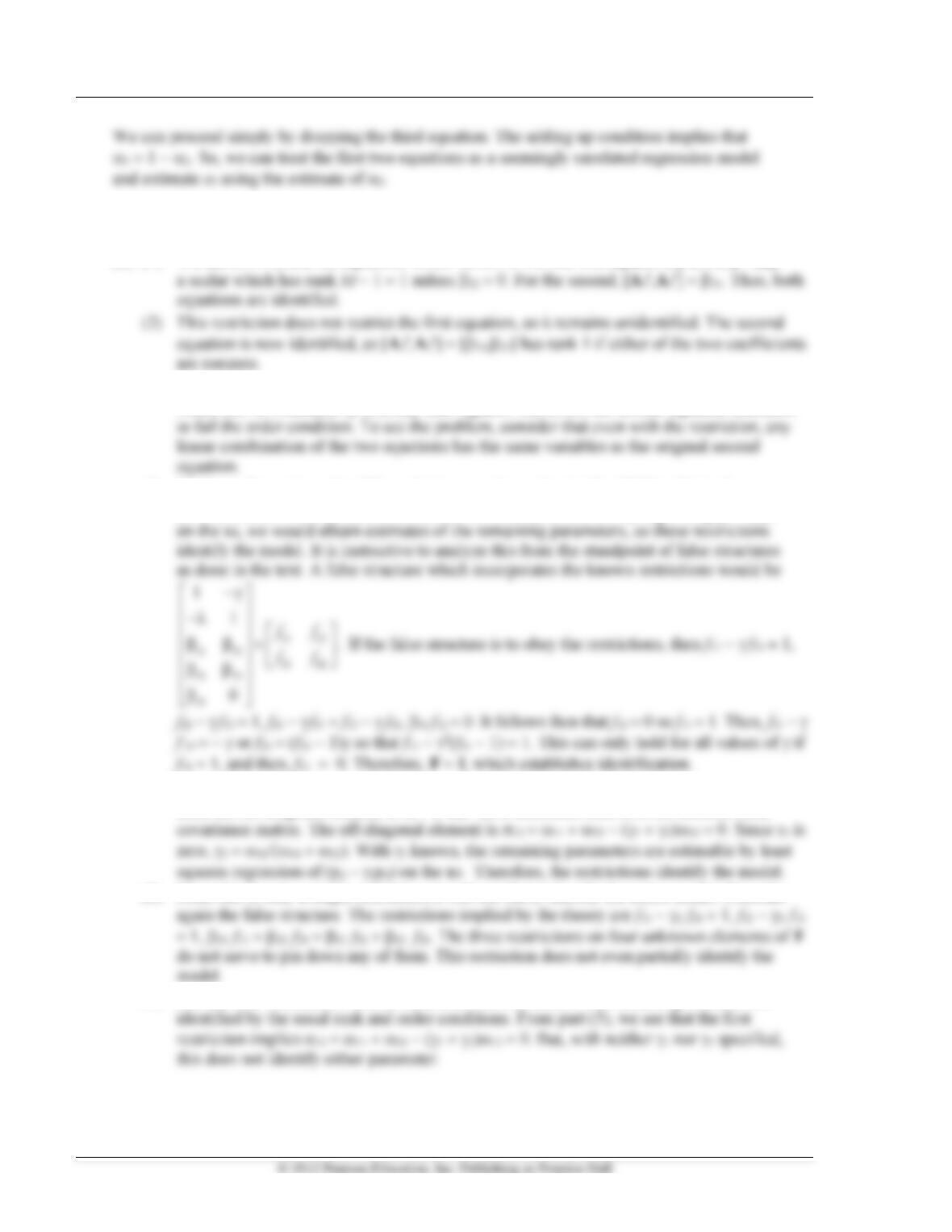
Proceeding directly, we obtain
1
0
q q y y
−
−
It remains only to multiply the matrices and collect terms. The result is
7. Once again, nothing is lost by assuming that
x
= 0. Now, the OLS estimators are
a1 =
1,y
a2 =
2,y
a3 =
3,y
b = xy1/xx.
The vector of residuals is ei1 = yi1 −
1
y
− bxi
80 Greene • Econometric Analysis, Seventh Edition
8. (a) Since nothing is excluded from either equation and there are no other restrictions, neither
equation passes the order condition for identification.
(b) (1) We use (13-12) and the equations which follow it. For the first equation, [A3,A5] = 22,
(3) If 1 equals 0, the model becomes partially recursive. The first equation becomes a regression
which can be estimated by ordinary least squares. However, the second equation continues
(4) We know from above that if 32 = 0, the second equation is identifiable. If it is, then
2 is identified. We may treat it as known. As such, 1 is known. By regressing y1 − 1y2
(5) If 31 = 0, the first equation is identified by the usual rank and order conditions. Consider,
then, the off-diagonal element of = . is identified since it is the reduced form
(6) Since this is only a single restriction, it will not likely identify the entire model. Consider
(7) The last four restrictions remove x2 and x3 from the model. The remaining model is not
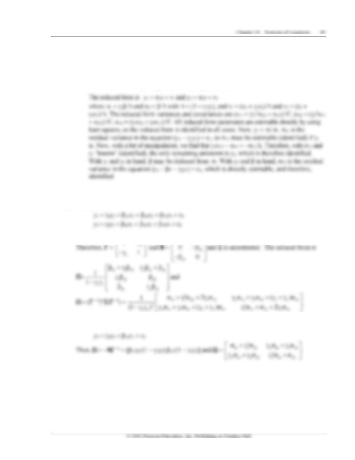
(8) The first equation is identified by the conventional rank and order conditions. The second
equation fails the order condition. But, the restriction 12 = 0 provides the necessary additional
information needed to identify the model. For simplicity, write the model with the restrictions
imposed as
y1 = 1y2 + 1 and y2 = 2y1 + x + 2.
9. Obtain the reduced form for the model in Exercise 1 under each of the assumptions made in parts (a),
(b1), and (b9).
(1) The model is
11 12
− −
(2) The model is
y1 = 1y2 + 1
82 Greene • Econometric Analysis, Seventh Edition
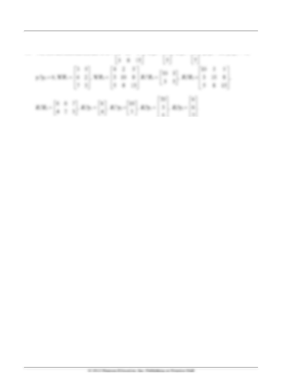
10. The relevant submatrices are XX =
7
6
5 2 3
2 10 8 ,
Xy1 =
4
3,
Xy2 =
3
6,
y1y1 = 20, y2y2 = 10,
5
7
Chapter 10 Systems of Equations 83
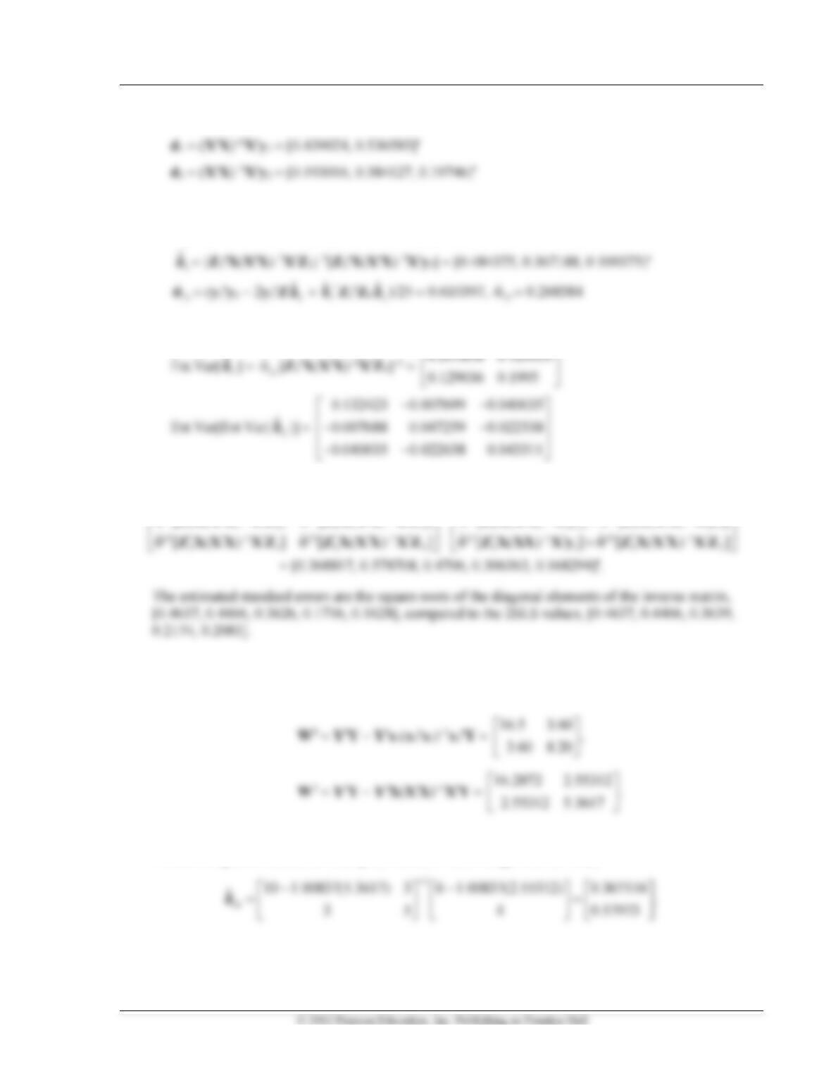
The two OLS coefficient vectors are
The two stage least squares estimators are
1
ˆ
= [Z1X(XX)−1XZ1]−1[Z1X(XX)−1Xy1] = [0.368816, 0.578711]
1
ˆ
The estimated asymptotic covariance matrices are
1
ˆ
The three stage least squares estimate is
1
11 1 12 1 11 1 12 1
ˆ ˆ ˆ ˆ
[ ( ) ] [ ( ) ] [ ( ) ] [ ( ) ]
−
− − − −
+
Z X X X X Z Z X X X X Z Z X X X X y Z X X X X y
To compute the limited information maximum likelihood estimator, we require the matrix of sums
of squares and cross products of residuals of the regressions of y1 and y2 on x1 and on x1, x2, and x3.
These are
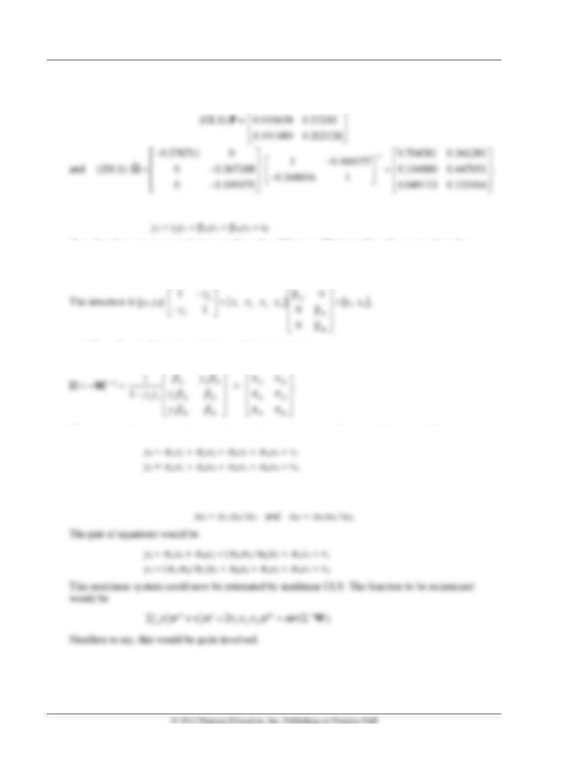
The two characteristic roots of (W1)−1W0 are 1.53157 and 1.00837. We carry the smaller one into the
k-class computation [see, for example, Theil (1971) or Judge et al. (1985)]:
84 Greene • Econometric Analysis, Seventh Edition
Finally, the two estimates of the reduced form are
0.680851 0.329787
11. For the model y1 = 1y2 + 11x1 + 21x2 + 1
show that there are two restrictions on the reduced form coefficients. Describe a procedure for
estimating the model while incorporating the restrictions.
11
0
or y + xB = . The reduced form coefficient matrix is
11 2 11
11 21
The two restrictions are 12/11 = 22/21 and
31/
32 =
41/
42. If we write the reduced form as
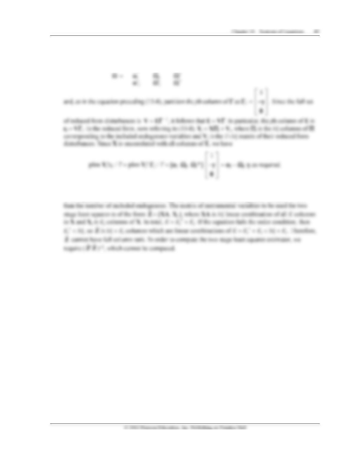
We could treat the system as a nonlinear seemingly unrelated regressions model. One possible way to
handle the restrictions is to eliminate two parameters directly by making the substitutions
12. Prove plim Yj/T = j − jj j.
Consistent with the partitioning y = [yj Yj Yi*], partition into
jj j *j
13. Prove that an underidentified equation cannot be estimated by two stage least squares.
If the equation fails the order condition, then the number of excluded exogenous variables is less