244
CASE STUDY EXTENSION
10–3 Are Prices Sticky? I: Evidence from Individual Transactions
1966.1 He looked at buyer–seller pairings—that is, cases in which a particular seller sold the same good to
a particular buyer on a number of successive occasions. A measure of price rigidity, then, is the number of
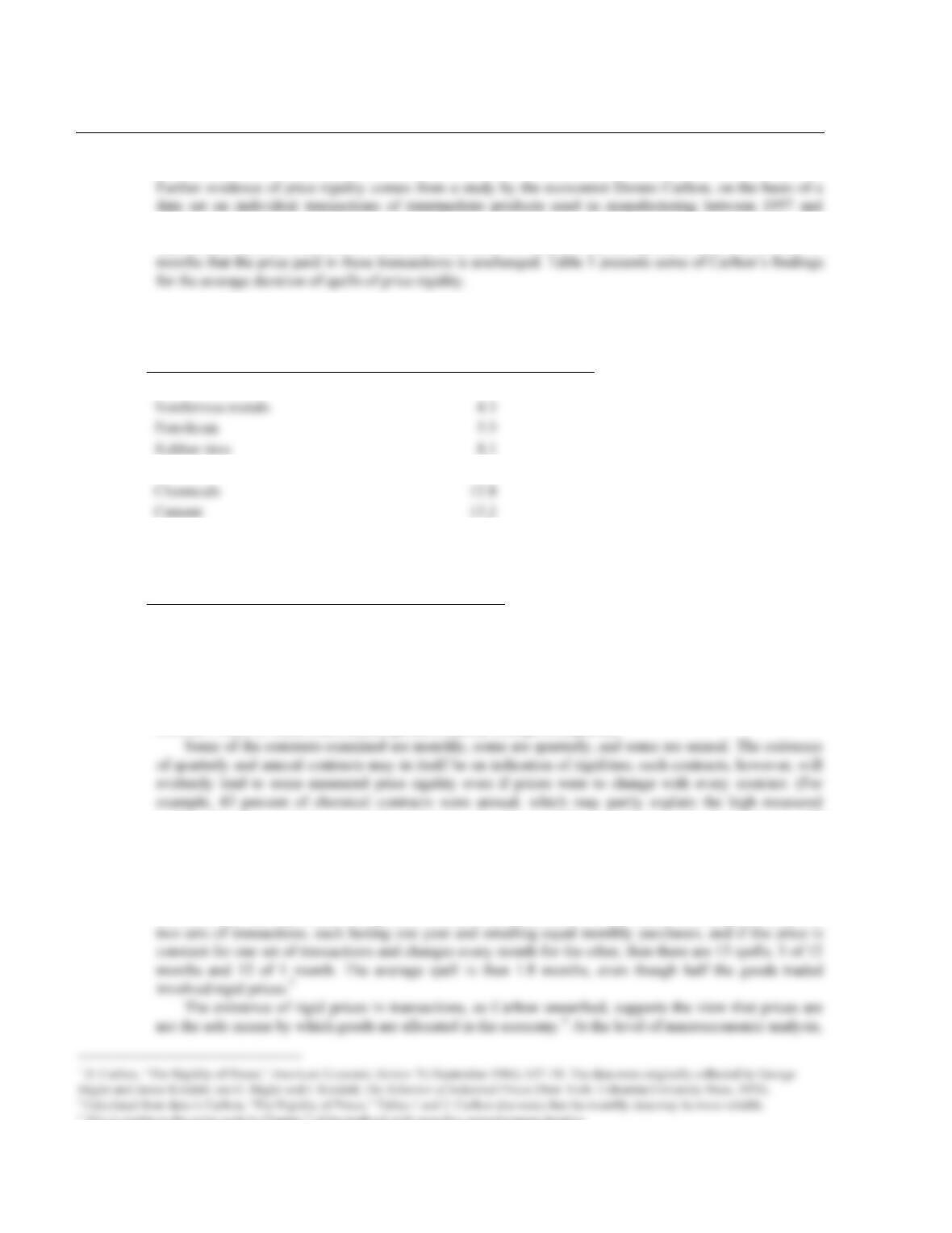
Table 1
Product Group
Average Duration of Price
Rigidity (months)
Steel
13.0
Nonferrous metals
4.3
8.1
Paper
8.7
12.8
13.2
Glass
10.2
Truck motors
5.4
Plywood
4.7
Household appliances
3.6
Average (weighted)
9.9
Source: Based on D. Carlton, “The Rigidity of Prices,” American Economic Review 76 (September 1986): 637–58.
These data provide strong support for the belief that prices exhibit substantial rigidity. In three
product groups (which account for more than half the buyer–seller pairings), the average rigidity of prices
is more than one year. The weighted average for the entire sample (of almost 1,900 pairings) is about ten
months. Prices for these intermediate goods evidently change infrequently.
rigidity for that product group.) Examination of only monthly contracts reveals that there is still
considerable evidence of price rigidity: the (weighted) average duration for monthly contracts is 7.2
months.2 Another interesting feature of the data is that there is a great deal of variation in duration spells
within product groups.
Measuring duration in terms of the average length of a pairing with rigid prices is likely to
underestimate the importance of rigidities in terms of transactions. To use Carlton’s example, if there are
4 Observed rigidity of prices does not itself prove a failure of the price system. For one thing, as Carlton points out, prices may sometimes be rigid
245
it suggests that an assumption of completely flexible prices may not be appropriate for short–run analysis.
Modern new Keynesian analysis emphasizes that it is unsatisfactory simply to assume that prices are rigid,
however; rather, we need to understand why people agree on contracts that specify the same price (or
246
CASE STUDY EXTENSIOIN
10–4 Are Prices Sticky? II: Mail–Order Evidence
Anil Kashyap studied the prices of products sold through retail catalogs by firms such as L.L. Bean.1 He
argues that mail–order catalogs are a good source of information on pricing behavior, even though there is
obviously some inherent rigidity in catalog prices. The data are unusually reliable because there is little
ambiguity about the price charged: it is possible to select goods that have hardly changed over several
decades, and other features of service (such as delivery time) are essentially constant.
The firms Kashyap studied had the opportunity to change their prices every six months, yet they often
247
ADVANCED TOPIC
10–5 Price Stickiness and Pareto Efficiency
The short–run model of the economy developed in Part IV of the textbook shows that economic
fluctuations are more easily explained if prices are sticky rather than perfectly flexible. The assumption of
sticky prices also has implications for the way we think about the costs of the business cycle and the
desirability of government policies aimed at stabilizing the economy. The reason is that economists have
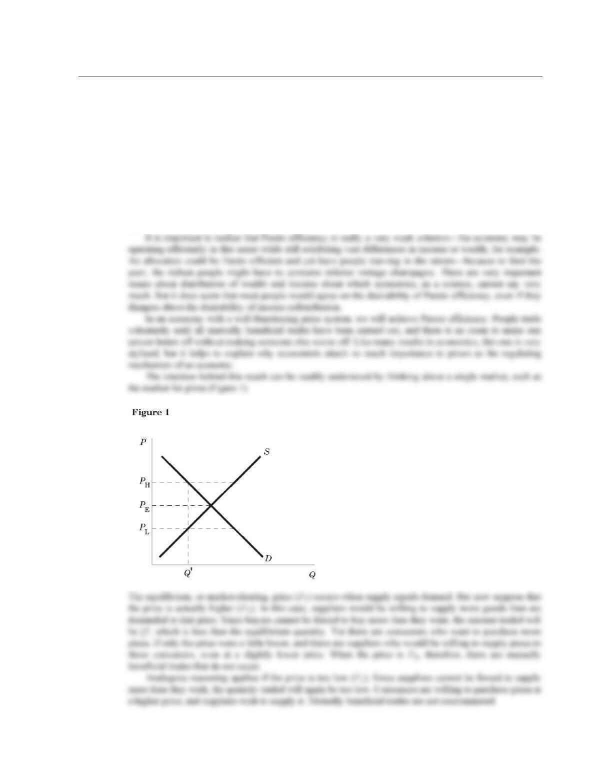
identified prices as the key regulating mechanism of the economy. Microeconomics teaches that prices
balance supply and demand and so help keep the economy functioning smoothly. In fact, a well–
functioning price system can achieve extraordinarily good results.
Economists pay a lot of attention to Pareto efficiency. We can think about the way goods and services
are allocated in the economy and ask: Is there any way of shifting goods around so that we can make some
people better off without making anyone else worse off? If not, we say that the allocation is Pareto
efficient. Otherwise, we say that it is inefficient.
248
Getting back to macroeconomics, this means that price stickiness not only helps to explain economic
fluctuations but also suggests that these fluctuations signal inefficiency. If sticky prices are at the root of
recessions and booms, then we might well believe that resources are being misallocated over the business
cycle. Consequently, we might also think that the government should intervene to stabilize the economy. If
all prices adjusted very quickly, conversely, this would suggest that the economy was doing as well as it
possibly could be, and there was no room for us to improve upon things by means of government policy.
(It could still be the case that we saw recessions, depressions, poverty, and the like; it might just be that we
couldn’t do anything about them.)
249
ADDITIONAL CASE STUDY
10–6 Velocity and the 1982 Recession
Is the velocity of money steady, or is it highly volatile? The answer to this question influences how the
Fed should conduct monetary policy. On the one hand, if velocity is steady, then it is easy to stabilize
aggregate demand: The Fed needs only to keep the money supply constant, or growing at a steady rate. On
the other hand, if velocity is highly volatile, then stabilizing aggregate demand requires adjusting the
money supply frequently to offset the changes in velocity.
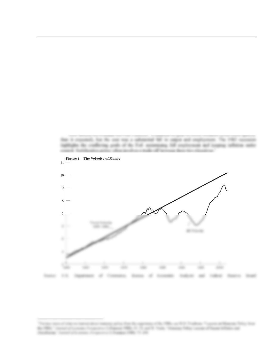
The deep recession that the United States experienced in 1982 is partly attributable to a large,
unexpected, and still mostly unexplained decline in velocity. Figure 1 graphs velocity (measured here as
nominal GDP divided by M1) from 1960 to 2000. The figure shows that velocity rose steadily in the 1960s
and 1970s but then fell markedly after 1981. The experience of the early 1980s shows that the Fed cannot
rely on the velocity of money remaining stable.
In 1982 the Fed could have offset the fall in velocity by raising the money supply. Containing
inflation was the Fed’s primary concern in the early 1980s, however, so it slowed the rate of money
growth instead, further depressing aggregate demand. The combination of these two forces—falling
velocity and anti–inflationary monetary policy—led to the deepest recession since the Great Depression of
the 1930s.
250
LECTURE SUPPLEMENT
10–7 Understanding Business Cycles II: Modeling Cycles
How do macroeconomists approach the problem of modeling the business cycle? One approach is to build
deterministic models that give rise to regular cyclical behavior. Early approaches to business cycles often
took this form; an example is Samuelson’s multiplier–accelerator model.1 But, as emphasized by Robert
Lucas, business cycles do not really appear to be characterized by the sort of smooth cyclical behavior
such models imply. Rather, business cycles occur at irregular intervals and are distinguished principally by
correlations (or co–movements) of different series. Modern business–cycle theory is thus not usually cast in
terms of such deterministic models.
The task of macroeconomists, broadly put, is to build models that match the stylized facts of the data.
But this task is complicated by a number of factors. First, there is not universal agreement on how best to
describe the data—in other words, we are not even completely sure of all the facts that we are trying to
explain. Second, there is disagreement on how best to judge a model’s ability to match the data. Third, we
do not know the relative importance of the different types of shock that hit the economy. Fourth, there is
disagreement about which propagation mechanisms are important.
One traditional approach to explaining the data is by the construction of large–scale macroeconometric
models (see Supplement 12-2). Some economists are skeptical of this approach, however, because such
models are subject to the Lucas critique (see Chapter 18) and so may be of limited use for policy analysis.
Another approach is that of real–business–cycle theorists (see Appendix to Chapter 9 and Supplement 15–
1). This approach emphasizes shocks to supply rather than demand and assumes that prices are flexible.
LECTURE SUPPLEMENT
10–8 The Economy in the Long Run and Very Long Run:
Summary of Parts II and III and Introduction to Part IV
Parts II and III of the textbook investigate the behavior of the economy in the long run and very long run;
we summarize that analysis here.
We first think about a large, closed economy. We wish to determine key macroeconomic variables—
more carefully in Part V of the textbook.) Equilibrium in the market for goods determines the equilibrium
real interest rate. Equally, this can be viewed as equilibrium in the market for loanable funds. Our analysis
up to this point has therefore considered the markets for capital, labor, and goods.
We have still not explained the determination of any nominal variables. We thus turn our attention to
the market for money and assume that the demand for real money balances depends on income and the
an economy. This means that it need no longer be the case that investment equal domestic saving; rather,
funds may come from abroad to finance our investment (negative net capital outflow); or, alternatively, we
may have domestic saving in excess of our needs for domestic investment (positive net capital outflow). In
the first case we are borrowing from abroad, hence consuming more than we are producing, hence running
a trade deficit (and conversely for the second case). The real exchange rate adjusts so as to keep the
run level of the capital stock, noting that, in a steady state, the capital–labor ratio is constant. The basis of
this analysis is that the dynamic behavior of the capital–labor ratio over time depends upon investment
(equivalently saving), which tends to increase the capital–labor ratio; and depreciation, population growth,
and technological progress, which all tend to decrease the capital–labor ratio. Our model of growth is
based on the same insight that underlies our model of income determination. In the background in our
worry about only four markets—capital, labor, goods, and money. Equilibrium in the capital and labor
markets is summarized by the long–run aggregate supply curve. Equilibrium in the goods and money
markets is summarized by the aggregate demand curve.
The long–run aggregate supply comes directly out of the previous long–run analysis. The aggregate
demand curve is a little trickier. The key point is that if Y is not pinned down (which it is not, since, in
long run hold in this analysis; it is simply a different way of representing the same ideas.
In the short run, though, we think that not all prices are flexible. Instead, we suppose that prices of
goods and services in the economy are sticky. The simplest way to summarize this idea is to suppose that
P is completely fixed in the short run. Firms set prices and then meet all demand. It thus no longer need be
the case that the markets for capital and labor are in equilibrium. We then summarize the short–run supply
ADDITIONAL CASE STUDY
10-9 The Cost of Business Cycles
A common presumption is that business cycles are costly. When the economy is in recession, there are
frequent calls for government action; and, as it would seem that resources are being wasted, that common
presumption might seem to make sense. Yet some have questioned whether business cycles are really so
bad.
It is hard to fault Lucas’s argument as far as it goes. But it can be argued that the costs of business
cycles involve far more than instability of consumption:
• The AD–AS model suggests that the business cycle consists of fluctuations around the natural rate of
output. Implicitly, it is assumed that there are fluctuations both above and below the natural rate, and
these are approximately equal in magnitude. To put it another way, the AS curve is viewed as
consumption fluctuation understates the consumption risk faced by a typical household.3 Second,
business cycles have distributional implications. If, as a society, we care particularly about the
welfare of the worst–off members, economic stabilization policies may be desirable.
• If, as many believe, sticky prices underlie business cycle fluctuations, then resources are being
misallocated. Instability of consumption is one manifestation of this inefficiency, but there are
LECTURE SUPPLEMENT
10–10 Additional Readings
Robert Lucas’s paper “Understanding Business Cycles” is a classic and very readable paper on the stylized
facts of macroeconomics and on the task facing macroeconomists: R. Lucas, “Understanding Business