Unlock document.
This document is partially blurred.
Unlock all pages and 1 million more documents.
Get Access
Questions for Review
1. The Keynesian-cross model tells us that fiscal policy has a multiplied effect on income.
The reason is that according to the consumption function, higher income causes higher
consumption. For example, an increase in government purchases of ΔGraises expendi-
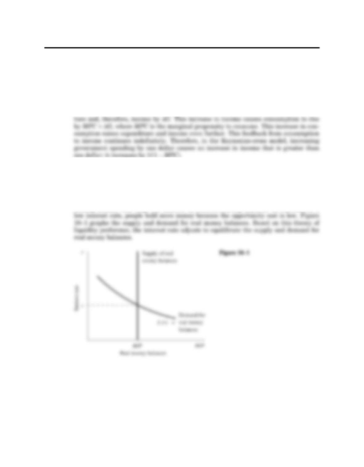
2. The theory of liquidity preference explains how the supply and demand for real money
balances determine the interest rate. A simple version of this theory assumes that
there is a fixed supply of money, which the Fed chooses. The price level Pis also fixed
in this model, so that the supply of real balances is fixed. The demand for real money
balances depends on the interest rate, which is the opportunity cost of holding money.
At a high interest rate, people hold less money because the opportunity cost is high. By
holding money, they forgo the interest on interest-bearing deposits. In contrast, at a
86
CHAPTER 10 Aggregate Demand I
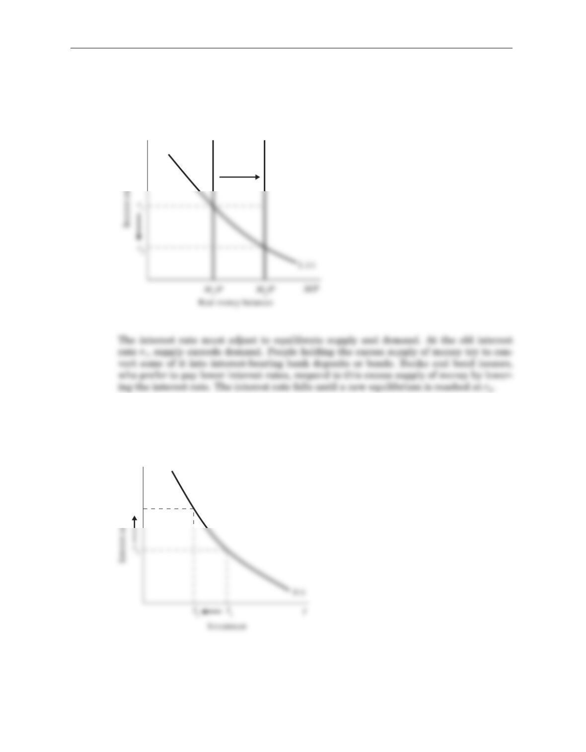
Why does an increase in the money supply lower the interest rate? Consider what
happens when the Fed increases the money supply from M1to M2. Because the price
level Pis fixed, this increase in the money supply shifts the supply of real money bal-
ances M/P to the right, as in Figure 10–2.
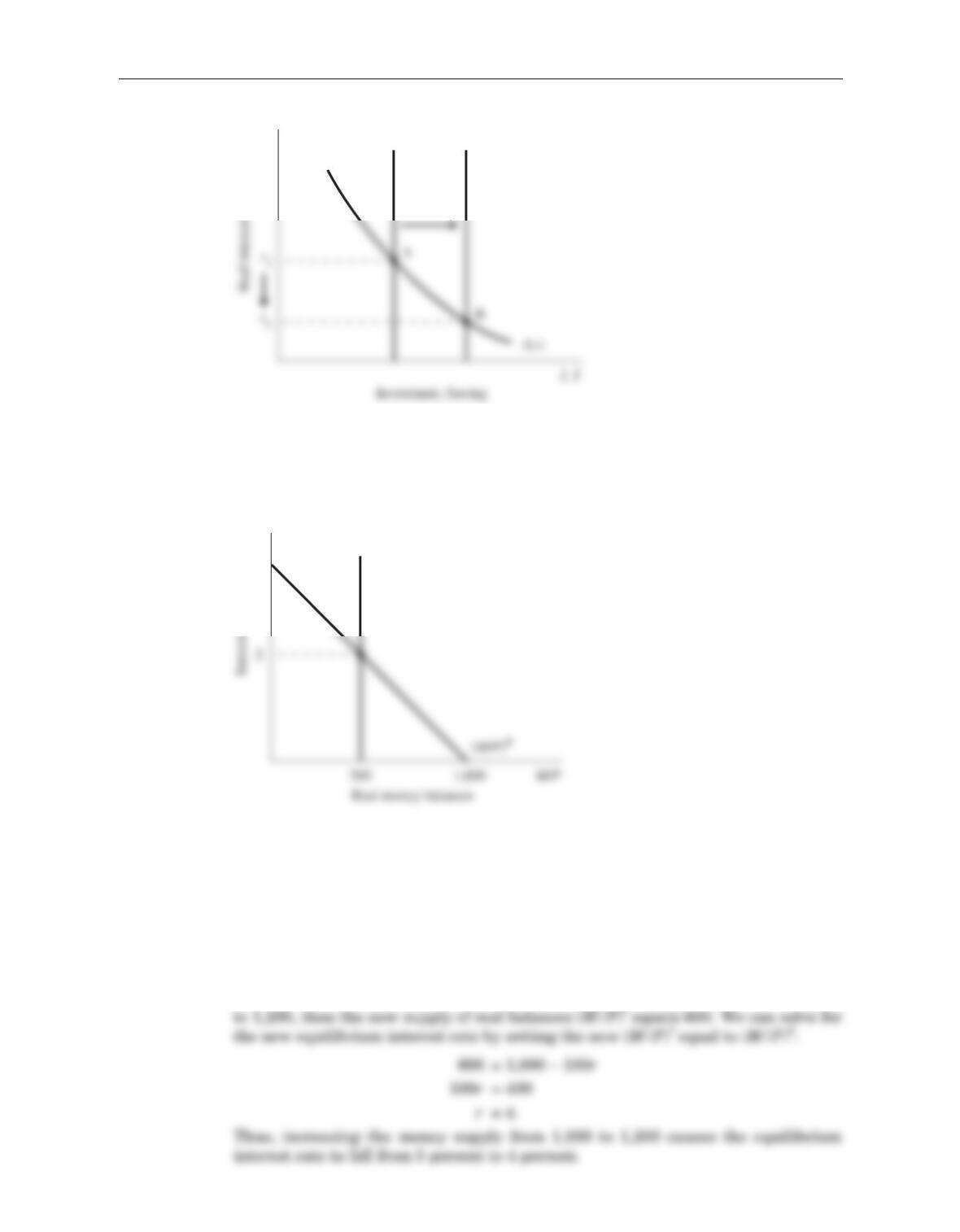
3. The IS curve summarizes the relationship between the interest rate and the level of
income that arises from equilibrium in the market for goods and services. Investment
is negatively related to the interest rate. As illustrated in Figure 10–3, if the interest
rate rises from r1to r2, the level of planned investment falls from I1to I2.
Chapter 10 Aggregate Demand I 87
r
Figure 10–2
r
r2
Figure 10–3
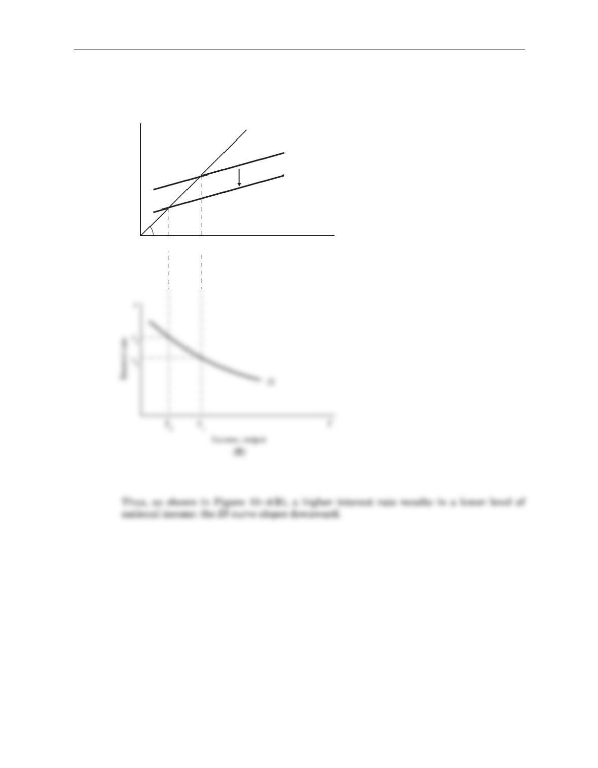
The Keynesian cross tells us that a reduction in planned investment shifts the expendi-
ture function downward and reduces national income, as in Figure 10–4(A).
88 Answers to Textbook Questions and Problems
45°
Planned expenditureInterest rate
YY2Y1
Y = PE
–
PE1 = C (Y T ) + I (r1) + G
–
PE2 = C (Y T ) + I (r2) + G
ΔI
Income, output
PE
(A)
Figure 10–4
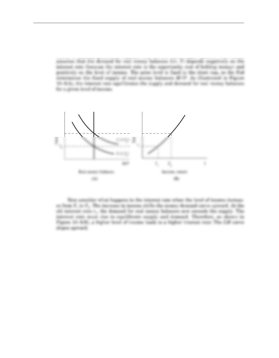
4. The LM curve summarizes the relationship between the level of income and the inter-
est rate that arises from equilibrium in the market for real money balances. It tells us
the interest rate that equilibrates the money market for any given level of income. The
theory of liquidity preference explains why the LM curve slopes upward. This theory
Chapter 10 Aggregate Demand I 89
r
r
M P/
LM
r2
r2
Figure 10–5
Problems and Applications
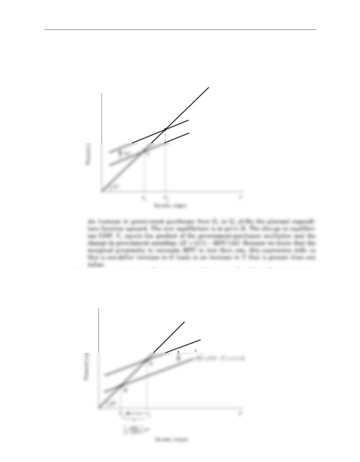
1. a. The Keynesian cross illustrates an economy’s planned expenditure function, PE =
C(Y– T) + I+ G, and the equilibrium condition that actual expenditure equals
planned expenditure, Y= PE, as shown in Figure 10–6.
b. An increase in taxes ΔTreduces disposable income Y– Tby ΔTand, therefore,
reduces consumption by MPC × ΔT. For any given level of income Y, planned
expenditure falls. In the Keynesian cross, the tax increase shifts the planned-
expenditure function down by MPC ×ΔT, as in Figure 10–7.
90 Answers to Textbook Questions and Problems
B
PE
PE2 = C(Y – T) + I + G2
PE1 = C(Y – T) + I + G1
Y = PE
Figure 10–6
Y = PE
MPC TΔ
PE
Figure 10–7
The amount by which equilibrium GDP falls is given by the product of the tax
multiplier and the increase in taxes:
ΔY= [ – MPC/(1 – MPC)]ΔT.
c. We can calculate the effect of an equal increase in government expenditure and
taxes by adding the two multiplier effects that we used in parts (a) and (b):
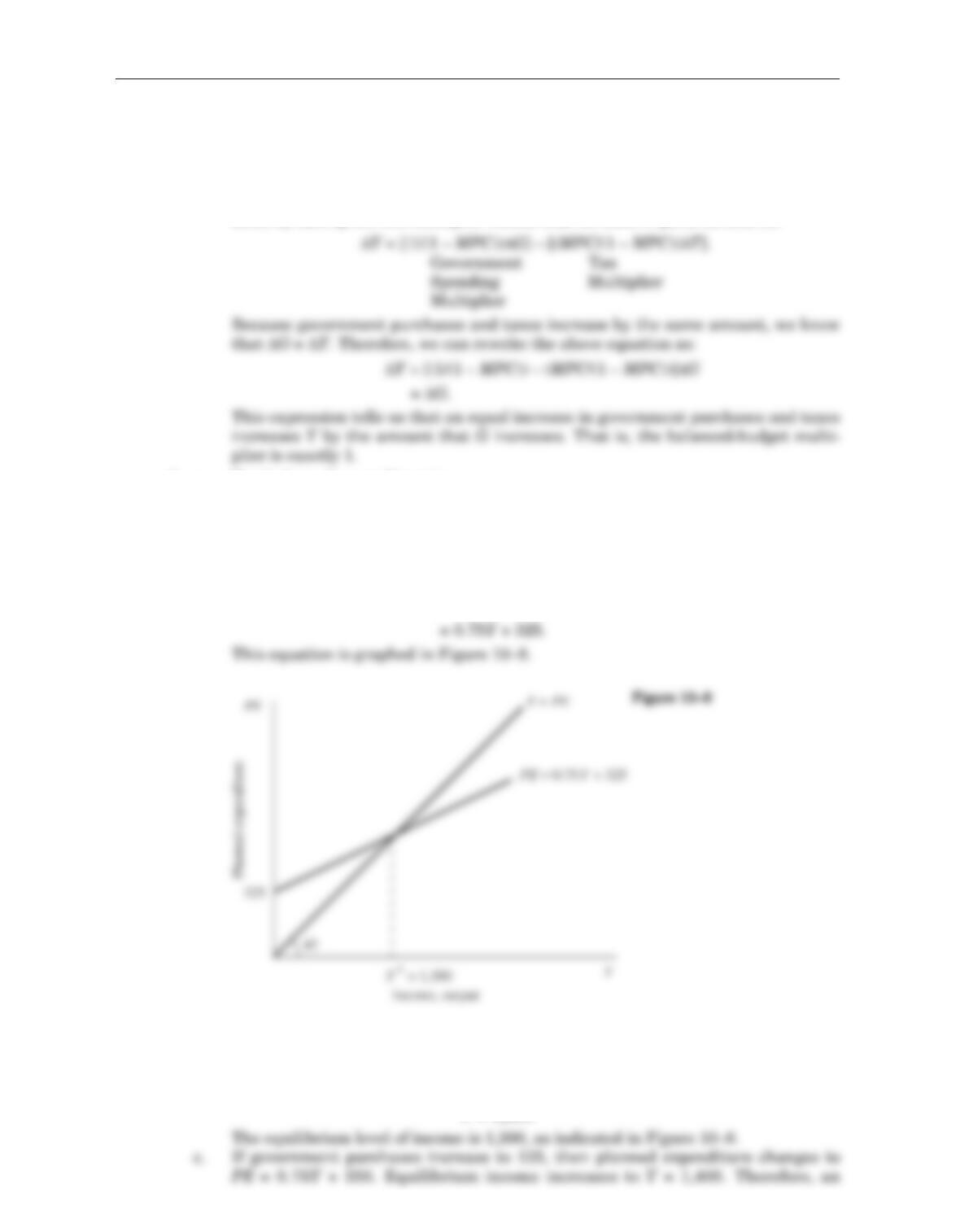
2. a. Total planned expenditure is
PE = C(Y– T) + I+ G.
Plugging in the consumption function and the values for investment I, govern-
ment purchases G, and taxes Tgiven in the question, total planned expenditure
PE is
PE = 200 + 0.75(Y– 100) + 100 + 100
b. To find the equilibrium level of income, combine the planned-expenditure equa-
tion derived in part (a) with the equilibrium condition Y= PE:
Y= 0.75Y+ 325
Y= 1,300.
Chapter 10 Aggregate Demand I 91
increase in government purchases of 25 (i.e., 125 – 100 = 25) increases income by
100. This is what we expect to find, because the formula for the government-pur-
chases multiplier
is 1/(1 – MPC), the MPC is 0.75, and the government-purchases
3. a. When taxes do not depend on income, a one-dollar increase in income means that
disposable income increases by one dollar. Consumption increases by the marginal
propensity to consume MPC. When taxes do depend on income, a one-dollar
increase in income means that disposable income increases by only (1 – t) dollars.
Consumption increases by the product of the MPC and the change in disposable
than dollar for dollar. Consumption then increases by an amount (1 – t)
MPC ×ΔG. Expenditure and income increase by this amount, which in turn caus-
es consumption to increase even more. The process continues, and the total
change in output is
ΔY= ΔG{1 + (1 – t)MPC + [(1 – t)MPC]2+ [(1 – t)MPC]3+ ....}
The consumption function is
C= a+ b(Y– T– tY).
Note that in this consumption function taxes are a function of income. The invest-
ment function is the same as in the chapter:
I= c– dr.
92 Answers to Textbook Questions and Problems
Î
˚
Chapter 10 Aggregate Demand I 93
The slope of the IS curve is therefore:
Recall that tis a number that is less than 1. As tbecomes a bigger number, the
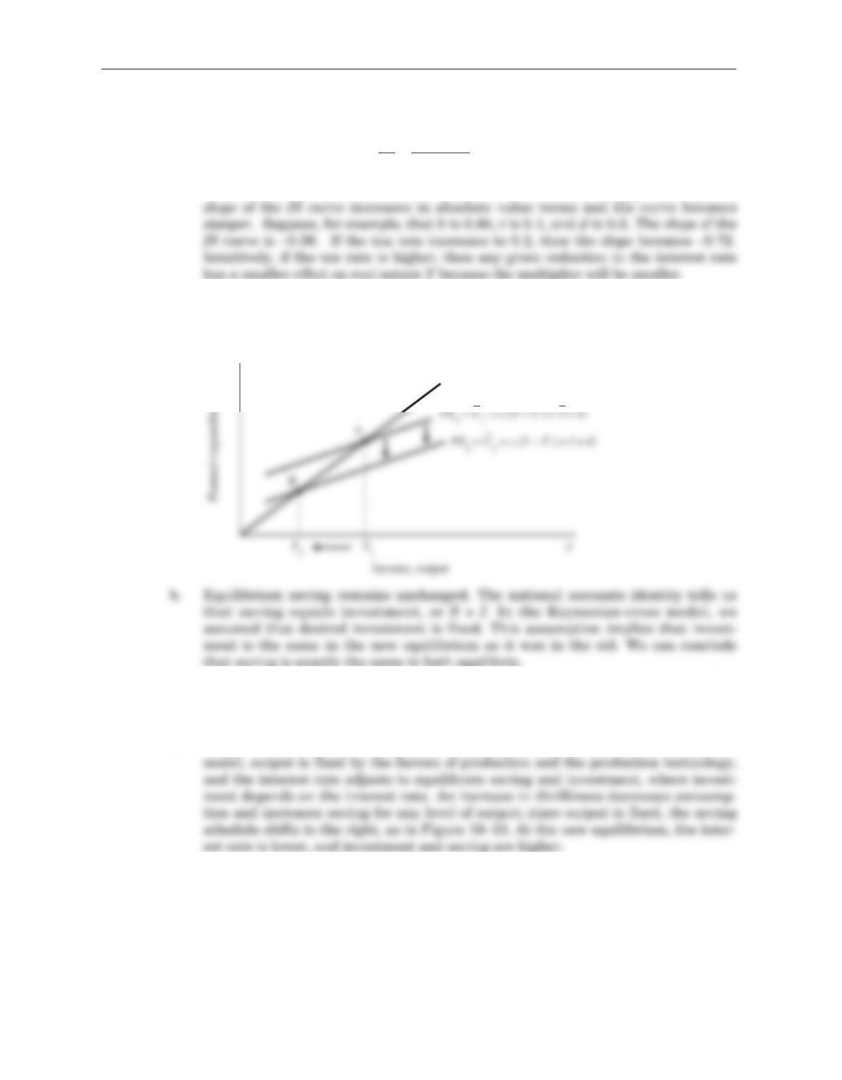
4. a. If society becomes more thrifty—meaning that for any given level of income people
save more and consume less—then the planned-expenditure function shifts down -
ward, as in Figure 10–9 (note that C2< C1). Equilibrium income falls from Y1to Y2.
c. The paradox of thrift is that even though thriftiness increases, saving is unaffect-
ed. Increased thriftiness leads only to a fall in income. For an individual, we usu-
ally consider thriftiness a virtue. From the perspective of the entire economy as
represented by the Keynesian-cross model, however, thriftiness is a vice.
d. In the classical model of Chapter 3, the paradox of thrift does not arise. In that
Y = PE
PE
Figure 10–9
D
D
r
y
bt
d
=-
()
-11
.
Thus, in the classical model, the paradox of thrift does not exist.
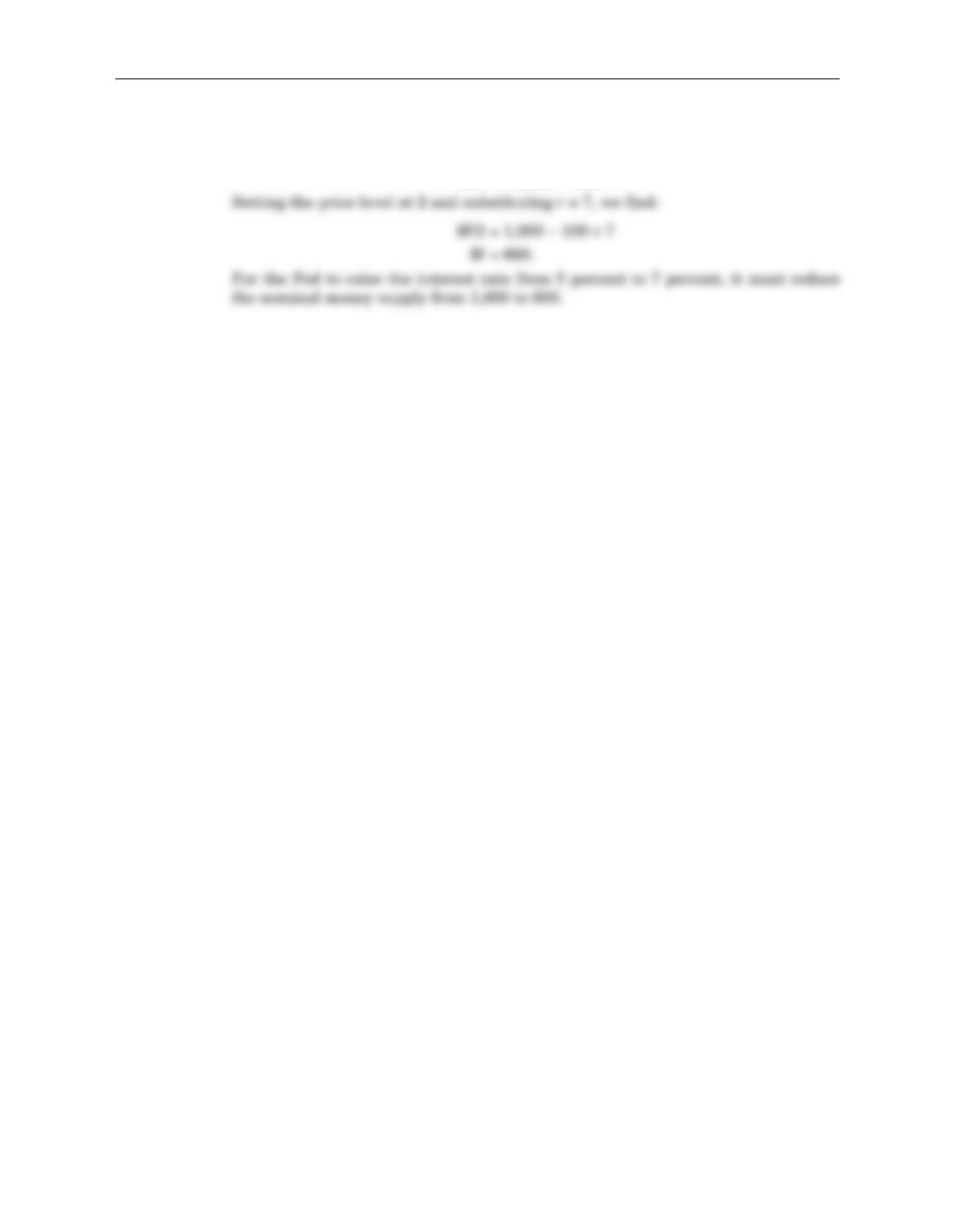
5. a. The downward sloping line in Figure 10–11 represents the money demand func-
tion (M/P)d= 1,000 – 100r. With M= 1,000 and P= 2, the real money supply
(M/P)s= 500. The real money supply is independent of the interest rate and is,
therefore, represented by the vertical line in Figure 10–11.
b. We can solve for the equilibrium interest rate by setting the supply and demand
for real balances equal to each other:
500= 1,000 – 100r
r= 5.
Therefore, the equilibrium real interest rate equals 5 percent.
c. If the price level remains fixed at 2 and the supply of money is raised from 1,000
94 Answers to Textbook Questions and Problems
r
10
(M/P)s
Figure 10–11
r
S2
S1
Figure 10–10
d. To determine at what level the Fed should set the money supply to raise the inter-
est rate to 7 percent, set (M/P)sequal to (M/P)d:
M/P = 1,000 – 100r.
Chapter 10 Aggregate Demand I 95


