117
CHAPTER 10
TEACHING NOTES
Because of its realism and its care in stating assumptions, this chapter puts a somewhat heavier
burden on the instructor and student than traditional treatments of time series regression.
I think it is useful to discuss static and finite distributed lag models at the same time, as these at
least have a shot at satisfying the Gauss-Markov assumptions. Many interesting examples have
distributed lag dynamics. In discussing the time series versions of the CLM assumptions, I rely
mostly on intuition. The notion of strict exogeneity is easy to discuss in terms of feedback. It is
also pretty apparent that, in many applications, there are likely to be some explanatory variables
that are not strictly exogenous. What the student should know is that, to conclude that OLS is
unbiased – as opposed to consistent – we need to assume a very strong form of exogeneity of the
regressors. Chapter 11 shows that only contemporaneous exogeneity is needed for consistency.
SOLUTIONS TO PROBLEMS
10.1 (i) Disagree. Most time series processes are correlated over time, and many of them
(ii) Agree. This follows immediately from Theorem 10.1. In particular, we do not need the
homoskedasticity and no serial correlation assumptions.
(iii) Disagree. Trending variables are used all the time as dependent variables in a regression
10.2 We follow the hint and write
Now by assumption, ut-1 has zero mean and is uncorrelated with all right-hand-side variables in
the previous equation, except itself of course. So
10.3 Write
y* =
119
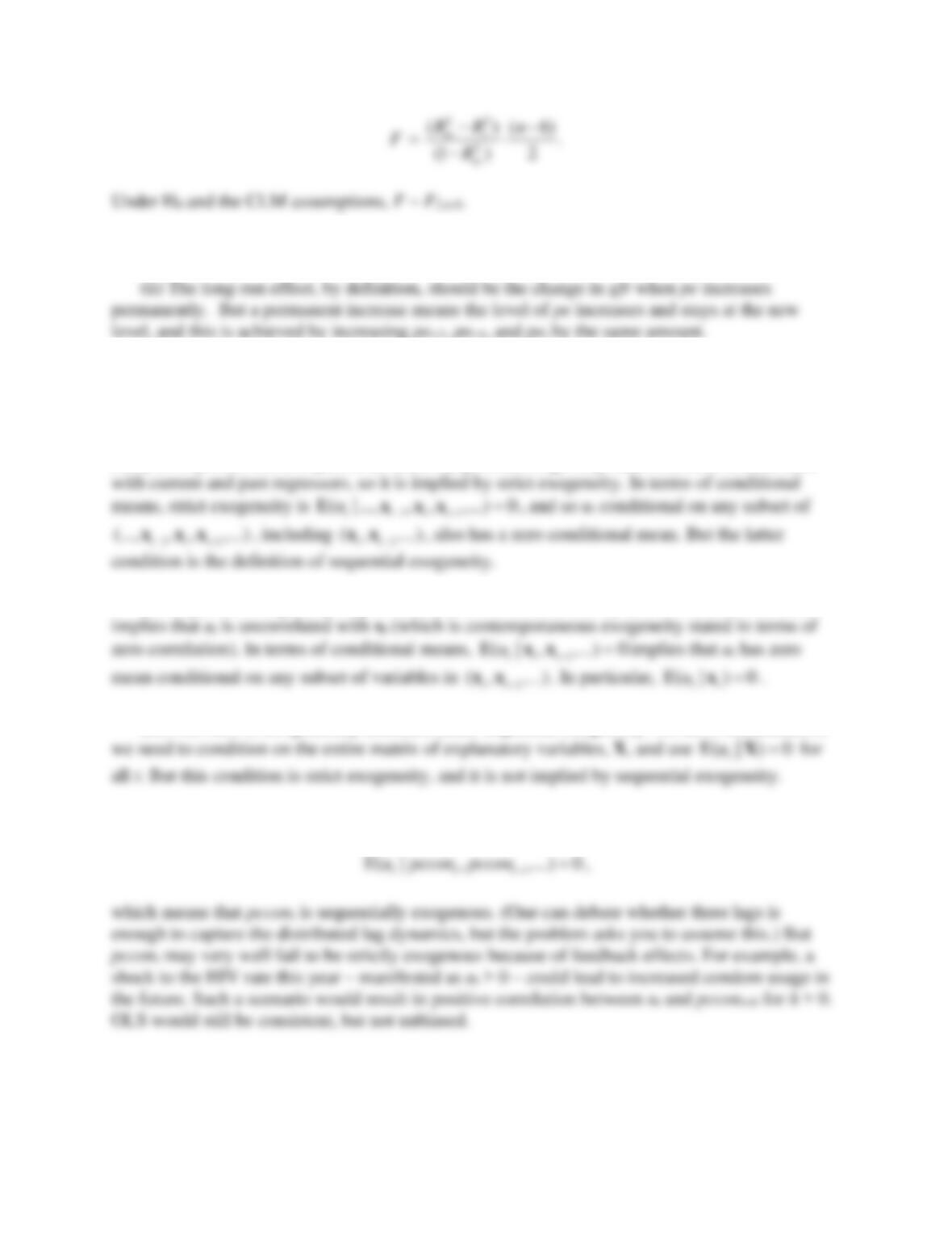
10.4 We use the R-squared form of the F statistic (and ignore the information on
2
R
). The 10%
critical value with 3 and 124 degrees of freedom is about 2.13 (using 120 denominator df in
10.5 The functional form was not specified, but a reasonable one is
10.6 (i) Given
j =
0 +
1 j +
2 j2 for j = 0,1, ,4, we can write
(ii) This is suggested in part (i). For clarity, define three new variables: zt0 = (zt + zt-1 + zt-2 +
(iii) The unrestricted model is the original equation, which has six parameters (
0 and the
five
j). The PDL model has four parameters. Therefore, there are two restrictions imposed in
120
10.7 (i) pet-1 and pet-2 must be increasing by the same amount as pet.
10.8 It is easiest to discuss this question in the context of correlations, rather than conditional
means. The solution here does both.
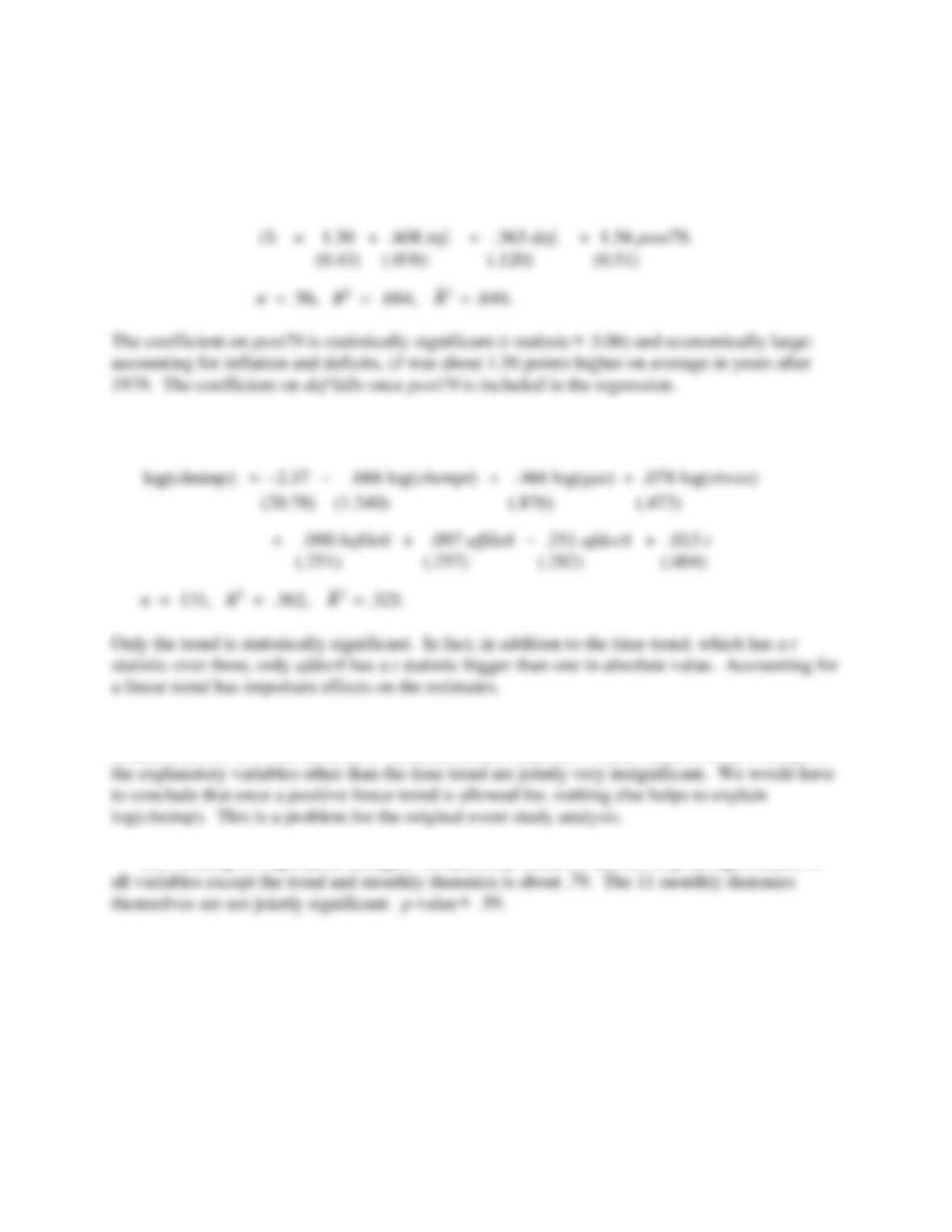
(i) Strict exogeneity implies that the error at time t, ut, is uncorrelated with the regressors in
every time period: current, past, and future. Sequential exogeneity states that ut is uncorrelated
(ii) Sequential exogeneity implies that ut is uncorrelated with xt, xt-1, …, which, of course,
(iii) No, OLS is not generally unbiased under sequential exogeneity. To show unbiasedness,
(iv) The model and assumption imply
121
SOLUTIONS TO COMPUTER EXERCISES
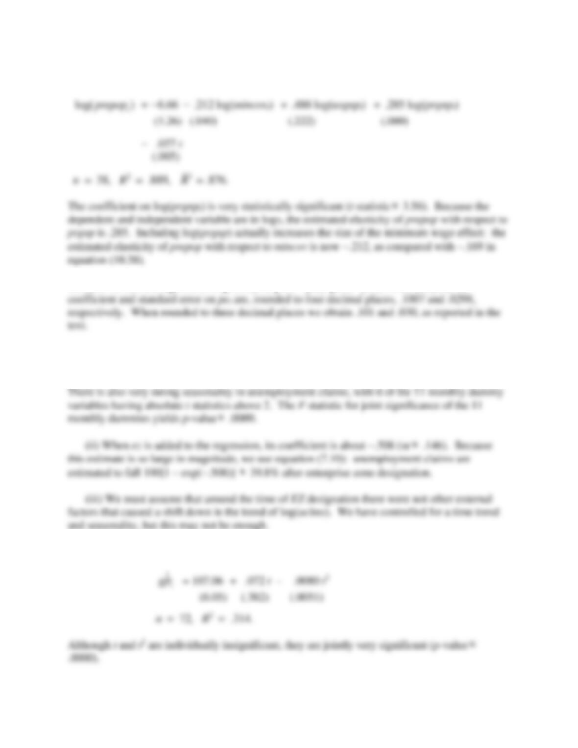
C10.1 Let post79 be a dummy variable equal to one for years after 1979, and zero otherwise.
Adding post79 to equation 10.15) gives
C10.2 (i) Adding a linear time trend to (10.22) gives
(ii) The F statistic for joint significance of all variables except the trend and intercept, of
course) is about .54. The df in the F distribution are 6 and 123. The p-value is about .78, and so
(iii) Nothing of importance changes. In fact, the p-value for the test of joint significance of
122
C10.3 Adding log(prgnp) to equation (10.38) gives
C10.4 If we run the regression of gfrt on pet, (pet-1 – pet), (pet-2 – pet), ww2t, and pillt, the
C10.5 (i) The coefficient on the time trend in the regression of log(uclms) on a linear time trend
and 11 monthly dummy variables is about −.0139 (se
.0012), which implies that monthly
unemployment claims fell by about 1.4% per month on average. The trend is very significant.
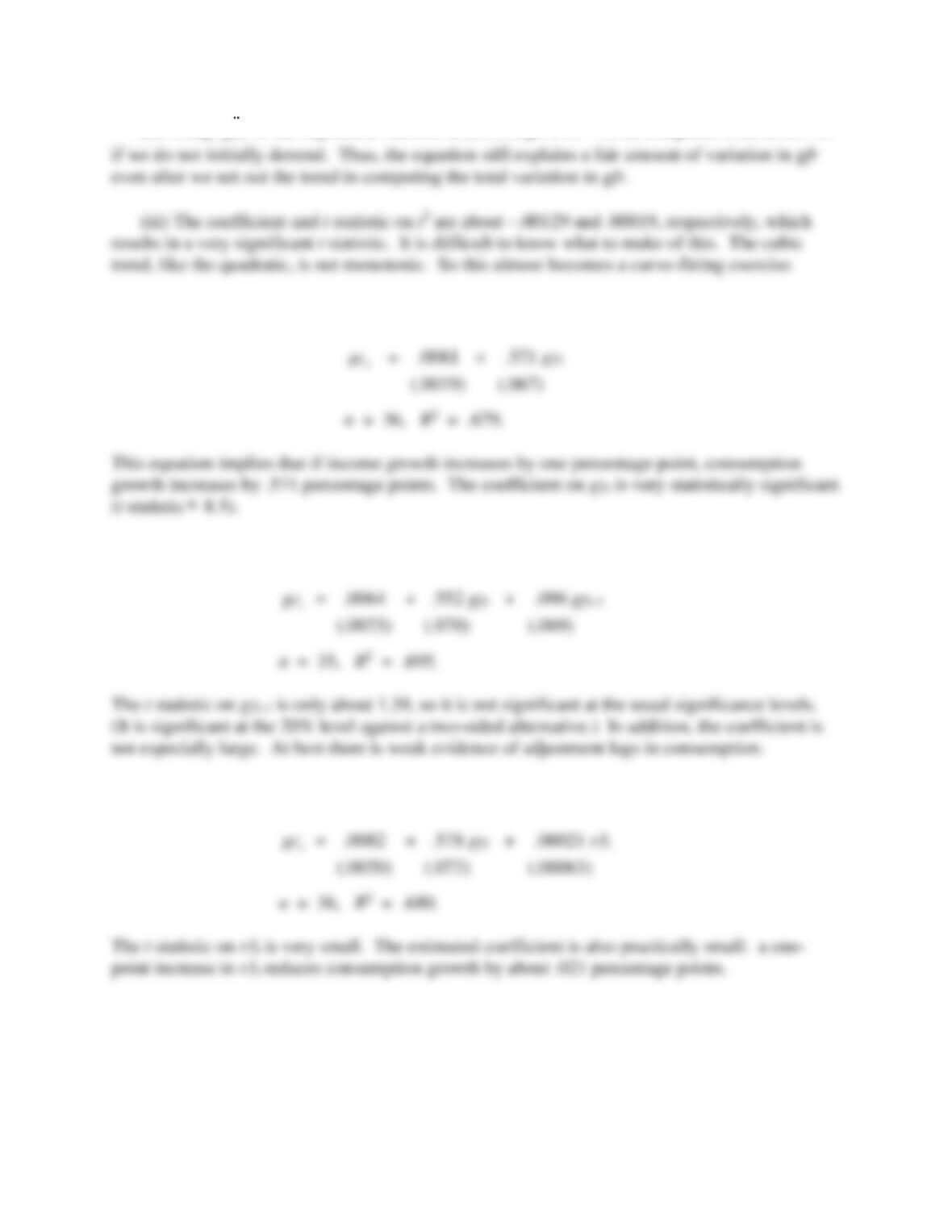
C10.6 (i) The regression of gfrt on a quadratic in time gives
123
(ii) Using
gfr
as the dependent variable in (10.35) gives R2
.602, compared with about .727
C10.7 (i) The estimated equation is
(ii) Adding gyt-1 to the equation gives
(iii) If we add r3t to the model estimated in part (i) we obtain
C10.8 (i) The estimated equation is
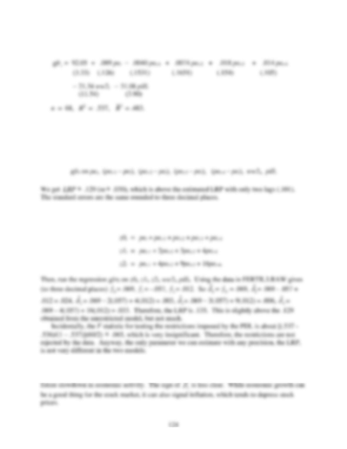
The p-value for the F statistic of joint significance of pet-3 and pet-4 is about .94, which is very
weak evidence against H0.
(ii) The LRP and its standard error can be obtained as the coefficient and standard error on
pet in the regression
(iii) We estimate the PDL with the additional variables ww22 and pillt. To estimate 0, 1,
and 2, we define the variables
C10.9 (i) The sign of
2
is fairly clear-cut: as interest rates rise, stock returns fall, so
2
< 0.
Higher interest rates imply that T-bill and bond investments are more attractive, and also signal a
125
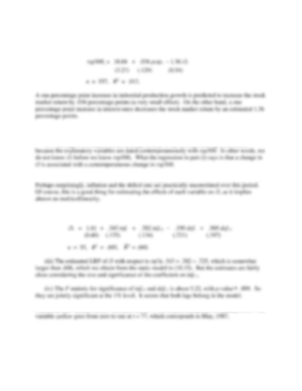
(ii) The estimated equation is
(iii) Only i3 is statistically significant with t statistic
−2.52.
(iv) The regression in part (i) has nothing directly to say about predicting stock returns
C10.10 (i) The sample correlation between inf and def is only about .098, which is pretty small.
(ii) The equation with the lags is
C10.11 (i) The variable beltlaw becomes one at t = 61, which corresponds to January, 1986. The
(ii) The OLS regression gives
126
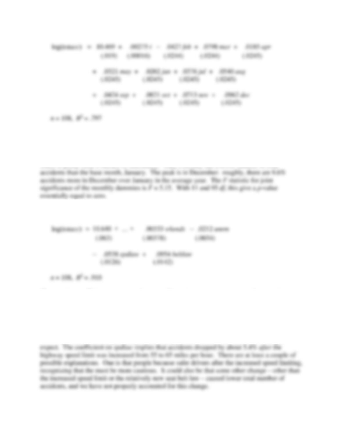
When multiplied by 100, the coefficient on t gives roughly the average monthly percentage
growth in totacc, ignoring seasonal factors. In other words, once seasonality is eliminated,
totacc grew by about .275% per month over this period, or, 12(.275) = 3.3% at an annual rate.
There is pretty clear evidence of seasonality. Only February has a lower number of total
(iii) I will report only the coefficients on the new variables:
The negative coefficient on unem makes sense if we view unem as a measure of economic
activity. As economic activity increases – unem decreases – we expect more driving, and
therefore more accidents. The estimate that a one percentage point increase in the
unemployment rate reduces total accidents by about 2.1%. A better economy does have costs in
terms of traffic accidents.
(iv) At least initially, the coefficients on spdlaw and beltlaw are not what we might
127
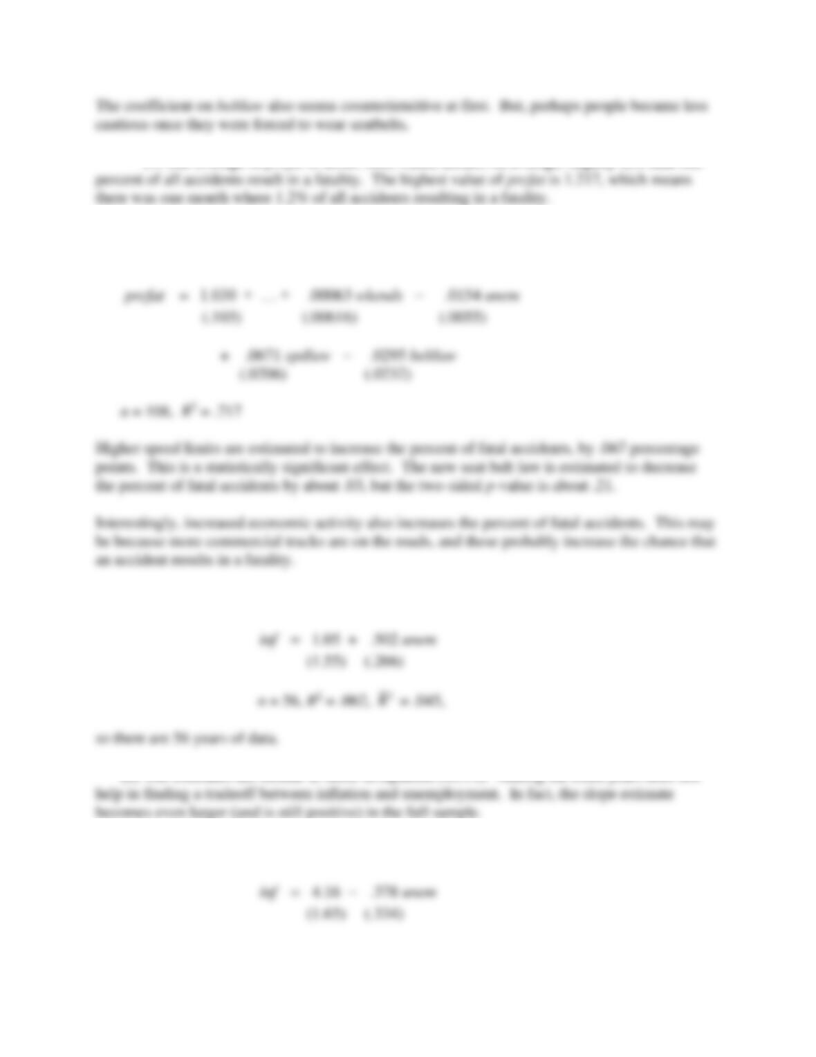
(v) The average of prcfat is about .886, which means, on average, slightly less than one
(vi) As in part (iii), I do not report the coefficients on the time trend and seasonal dummy
variables:
C10.12 (i) OLS estimation using all of the data gives
(ii) The estimates are similar to those in equation (10.14). Adding the extra years does not
(iii) Using only data from 1997 to 2003 gives
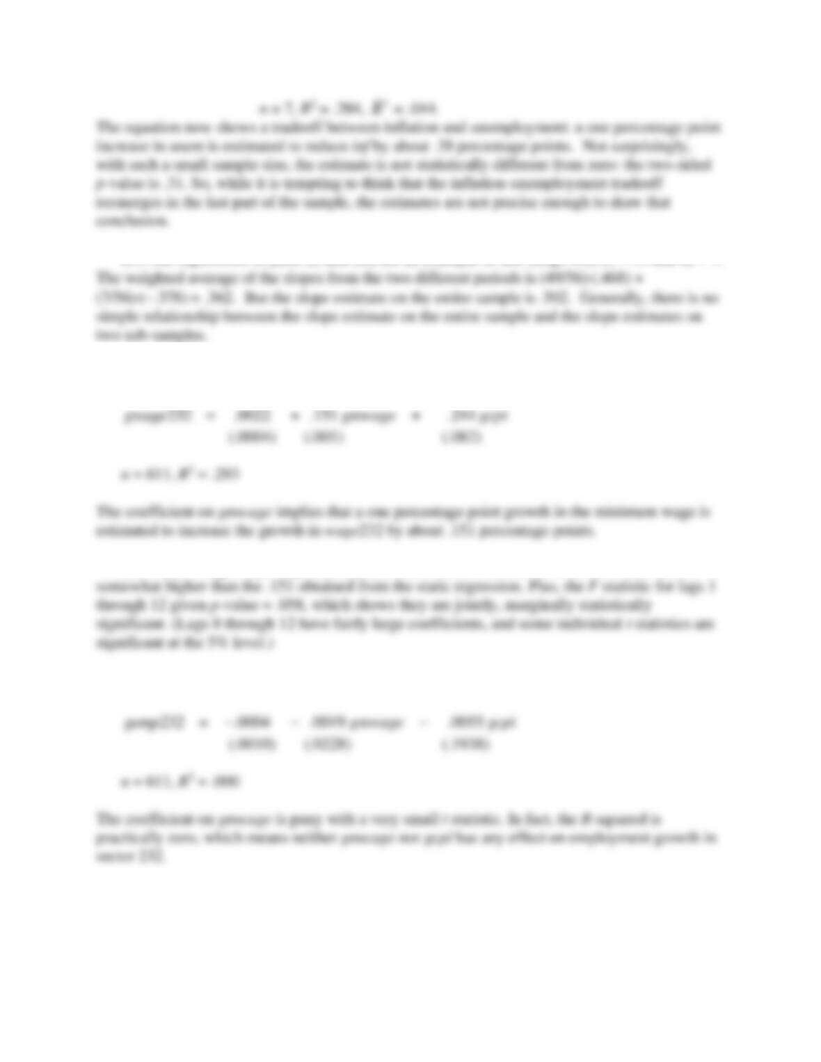
128
(iv) The regressions in parts (i) and (iii) are an example of this setup, with n1 = 49 and n2 = 7.
C10.13 (i) The estimated equation is
(ii) When 12 lags of gmwage are added, the sum of all coefficients is about .198, which is
(iii) The estimated equation is
(iv) Adding lags of gmwage does not change the basic story. The F test of joint significance
of gmwage and lags 1 through 12 of gmwage gives p-value = .439. The coefficients change sign
and none is individually statistically significant at the 5% level. Therefore, there is little evidence