Unlock document.
This document is partially blurred.
Unlock all pages and 1 million more documents.
Get Access

Answers to Selected
Student Guide Problems*
Data Questions
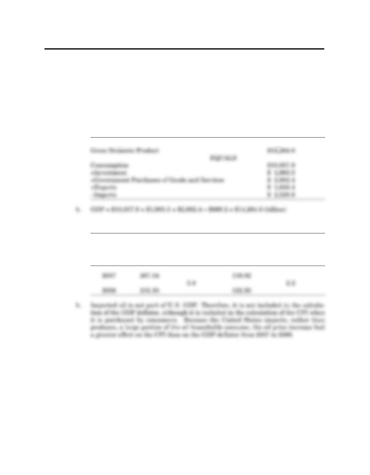
1. a. The following 2008 data, in billions of dollars, were obtained from the Bureau of
Economic Analysis Web site at http://www.bea.gov/. The data may be revised in
future publications.
Table 2–7
(1) (2)
2. a. Table 2–8
(1) (2) (3) (4) (5)
% Change % Change
in CPI from GDP in GDP Deflator from
Year CPI Preceding Year Deflator Preceding Year
203
CHAPTER 2The Data of Macroeconomics
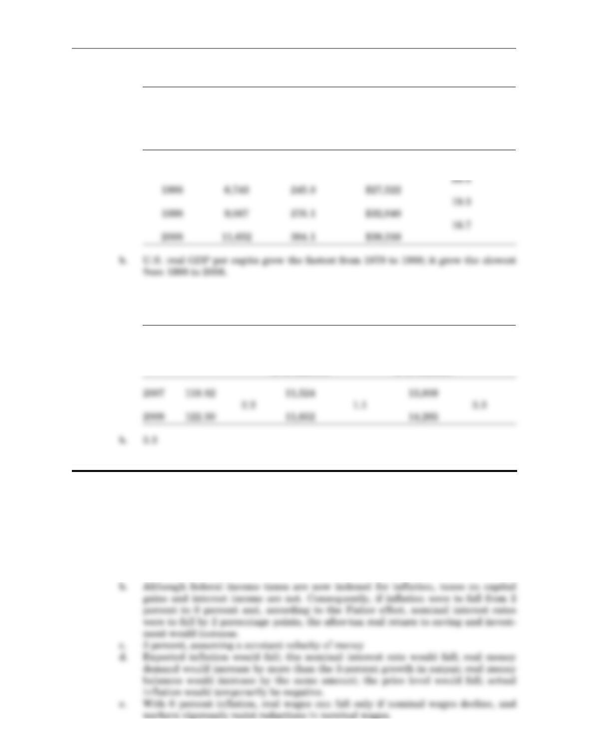
3. a. Table 2–9
(1) (2) (3) (4) (5)
% Change
Total U.S. in Real GDP
Real GDP Population Real GDP per Capita from
Year ($ in billions) (in millions) per Capita Preceding Decade
1978 5,015 222.6 $22,530
4. a. and c.
Table 2–10
(1) (2) (3) (4) (5) (6) (7)
GDP % Change Real % Change Nominal % Change
Year Deflator (P)in PGDP (Y)in YGDP (Y)in PY
($ in billions) ($ in billions)
Problems
10. a. The costs of expected inflation are the shoeleather costs of inflation, the menu
costs of changing prices, the cost of unindexed taxes, the cost of greater variability
in prices, and the costs to people who receive incomes fixed in nominal terms (such
as private pensions) that were contracted before the inflation was expected.
204 Answers to Selected Student Guide Problems
CHAPTER 4Money and Inflation
Data Questions
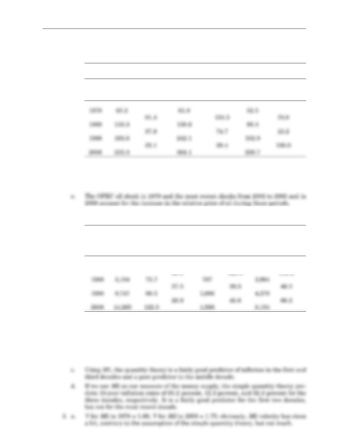
1. a. Table 4–9
(1) (2) (3) (4) (5) (6) (7)
Consumer Price Indices
CPI CPI
All % Medical % CPI %
Year Items Change Care Change Energy Change
b. $8.49
c. 1978 to 1988
d. 1998 to 2008
2. a. Table 4–10
(1) (2) (3) (4) (5) (6) (7) (8)
Nominal % Change M1(Dec.) M2(Dec.)
GDP($ in GDP in GDP ($ in % Change ($ in % Change
Year billions) Deflator Deflator billions) in M1 billions) in M2
1978 2,295 45.8 357 1,366
b. If the long-run growth rate of real GDP is 3 percent per year, or about 34 percent
per decade, and velocity were constant, the quantity theory would predict that
π= % Change in M – 34% per decade.
If we use
M
1 as our measure of the money supply, the simple quantity theory pre-
dicts 10-year inflation rates of 86.4 percent from 1978 to 1988; 5.3 percent from
1988 to 1998, and 11.6 percent from 1998 to 2008.
Chapter 4Money and Inflation 205
b.
V
for
M
1 in 1978 = 6.43,
V
for
M
1 in 2008 = 8.94;
M
1 velocity has risen a lot, con-
trary to the assumption of the simple quantity theory.
c. Even if velocity changes,
MV
=
PY
and the % change in
M
+ % change in
V
approximately equals the % change in
P
+ % change in
Y.
Thus, if both velocity
and real GDP change steadily over time, % change in
P
= % change in
M
+ %
change in
Y
– % change in
V
, and any increase in the money supply will be accom-
panied by an equal increase in the price level.
Problems
11. a. If the deficit were eliminated, public saving would rise. If taxes were cut, in the
long run private saving would also rise. Thus, national saving would rise.
b. In a closed economy, the S curve shifts right (as saving increases), the real rate of
interest falls, and the amount of investment increases although the investment
curve does not shift:
206 Answers to Selected Student Guide Problems
CHAPTER 5The Open Economy
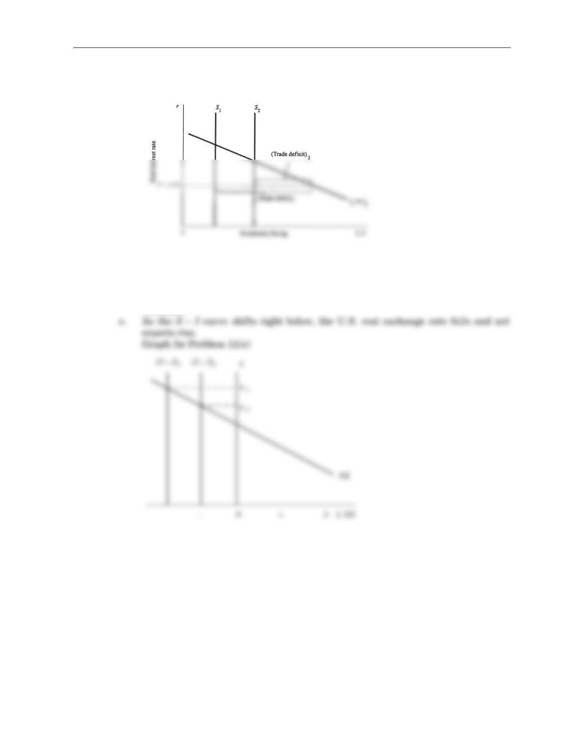
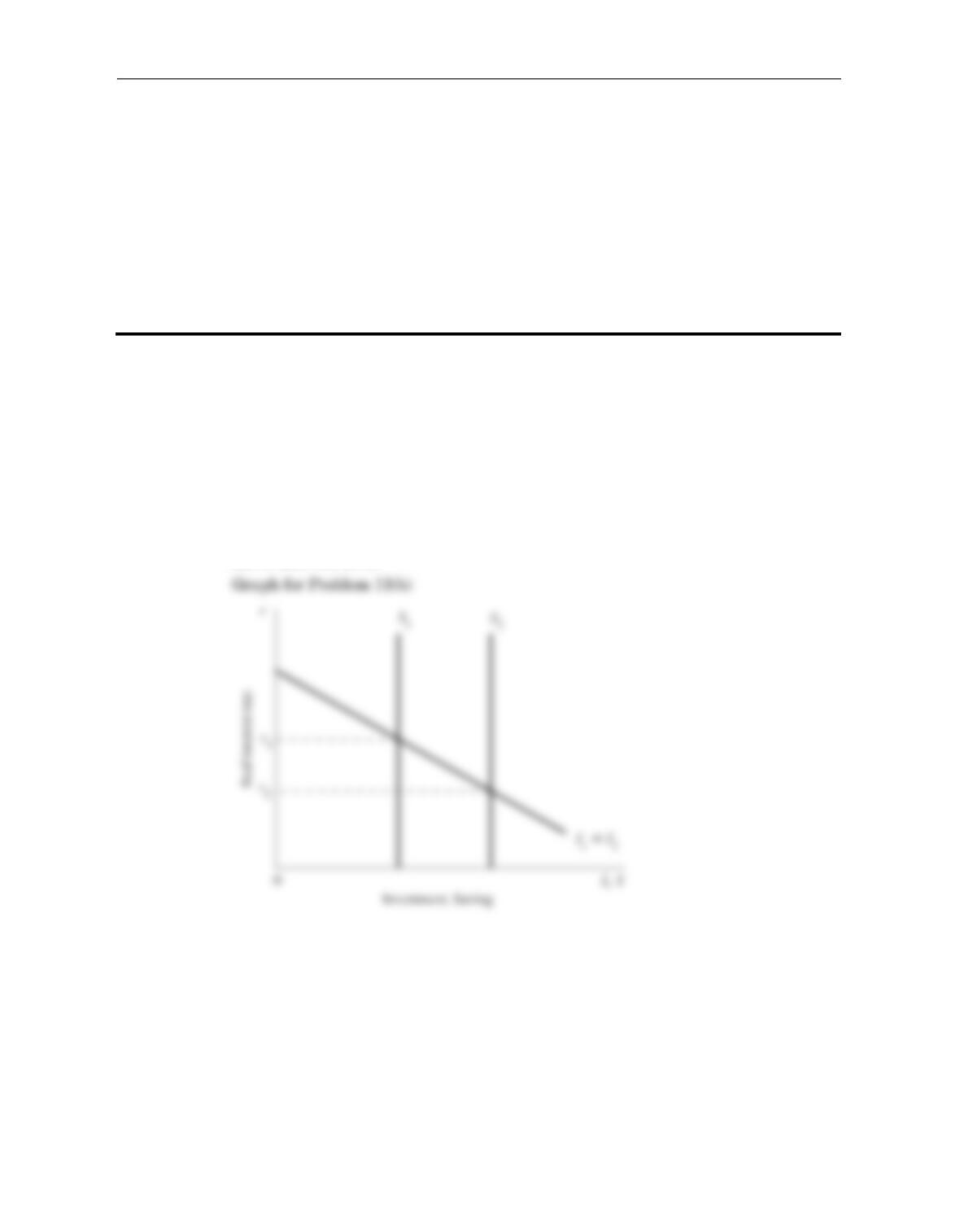
c. Graph for Problems 11(c) and 11(d)
d. Treating the United States as a small open economy, we once again shift the S
curve to the right as national saving increases. The real interest rate, however,
remains fixed at r*. Consequently, investment does not change, but S– I
increases.
Chapter 5The Open Economy 207
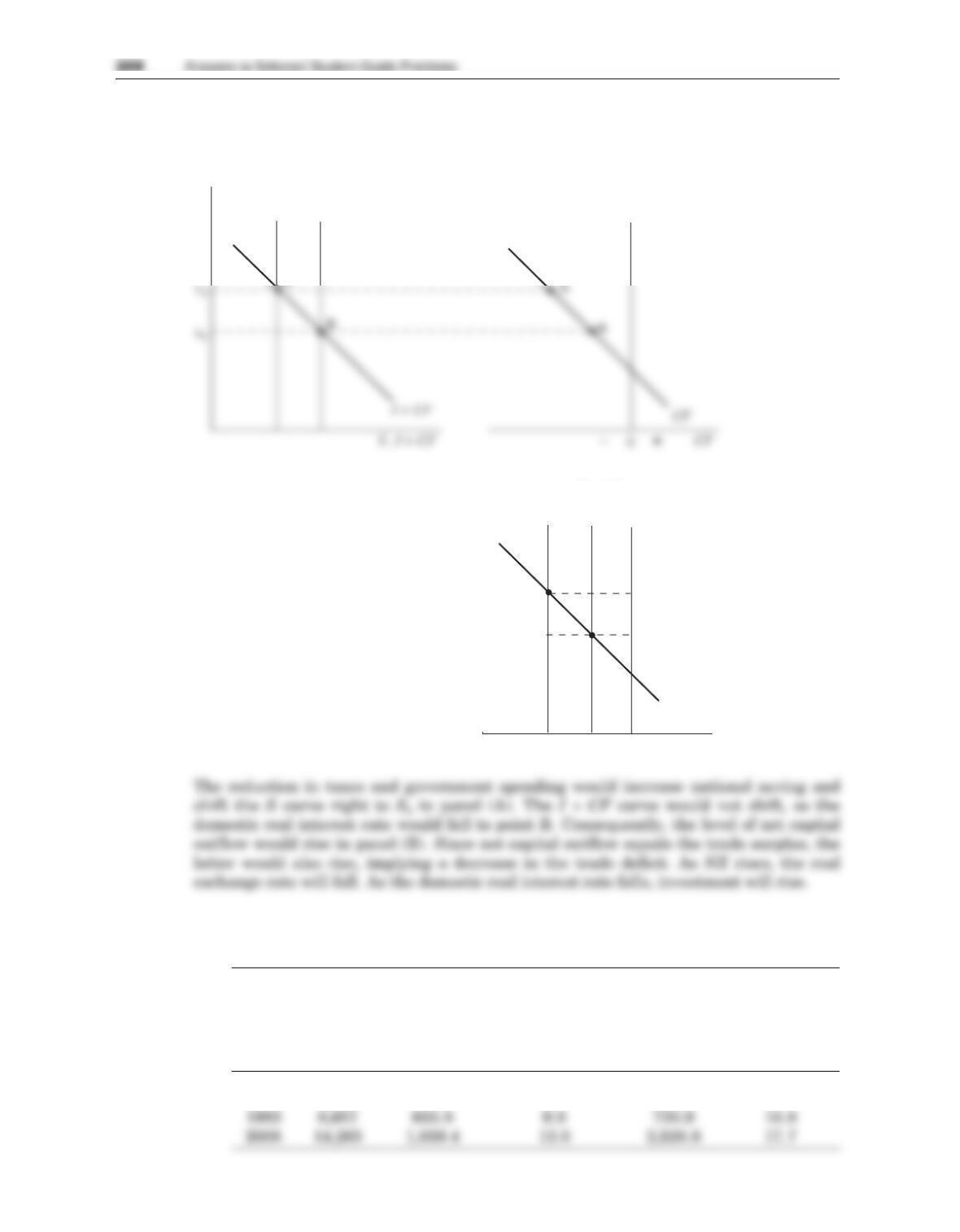
17. The initial equilibrium is represented by points A in panels (A), (B), and (C) below.
Graph for Problem 17
Data Questions
1. a. Table 5–8
(1) (2) (3) (4) (5) (6)
Exports of Imports of
Nominal Goods and Exports as Goods and Imports as
GDP ($ in Services % of Services % of
Year billions) ($ in billions) Nominal GDP ($ in billions) Nominal GDP
1978 2,295 186.9 8.1 212.3 9.3
Panel anel B
A
S1S2
r
Panel C
B
A
NX
NX
CF
rACF
rB
P
A
r
0+–
ε
ε
A
ε
B
c. Table 5–9
(1) (2) (3)
Net Exports of Goods Net Exports as
Year and Services ($ in billions) % of Nominal GDP
1978 –25.4 –1.1
3. a. The Western European natural rate of unemployment in the 1960s was 2.5 per-
cent, compared with the U.S. natural rate in the textbook of 4.76 percent.
b. 8 percent
6. a. E/POP = E/L ×L/POP, where POP = the noninstitutional population.
b. E/POP indicates the portion of the population that has a job. In a healthy econo-
Data Questions
1. a. Table 6–2
Labor-Force Participation Rates (in percent)
(1) (2) (3) (4)
Male and Female
Year Total Civilian Civilian Males Civilian Females
1968 59.6 80.1 41.6
Chapter 6Unemployment 209
CHAPTER 6Unemployment
c. Real GDP has risen by the amount of extra output women produce in their new
jobs. “Total production” does not rise as much as measured real GDP because the
reduction in household production that was formerly performed by these women
must be subtracted from the extra output produced in paid employment, especial-
ly between 1968 and 1988. If we consider the fact that many of these women now
pay others to do some of this household production, the difference between the
change in real GDP and the change in “total production” is even greater.
2. a. The median of a group of numbers is the “middle” number. Half of the numbers
are greater than the median, and half are less than the median. The mean or
3. a., b., and c.
Table 6–3
(1) (2) (3) (4) (5)
Inflation Conventional New
Unemployment Rate Misery Misery
Year Rate (Year to Year) Index Index
2006 4.6% 3.2% 7.8 11.0
Data Questions
1. a. Approximate Average Annual Percentage Growth Rates of Real GDP
1990–1999 2000–2008
United States 3.1 2.4
Japan 1.5 1.6
210 Answers to Selected Student Guide Problems
CHAPTER 7Economic Growth I
Problems
4. The short-run aggregate supply curve would shift downward, while the aggregate demand
curve would be unaffected. Output would rise, and the aggregate price level would fall.
Data Questions
1. a. Table 9–4
(1) (2) (3)
1979 1982 % Change
(in 1,000s) (in 1,000s) 1979–1982
Civilian noninstitutional population 164,863 172,271 4.5
Civilian labor force 104,962 110,204 5.0
c. The actual unemployment rate would eventually have equaled 5.8 percent.
2. In April 2009, the unemployment rate was 8.9 percent. If the unemployment rate for
all of 2009 was 8.9 percent, Okun’s law would predict that the real GDP would fall by
3.2 percent.
Problems
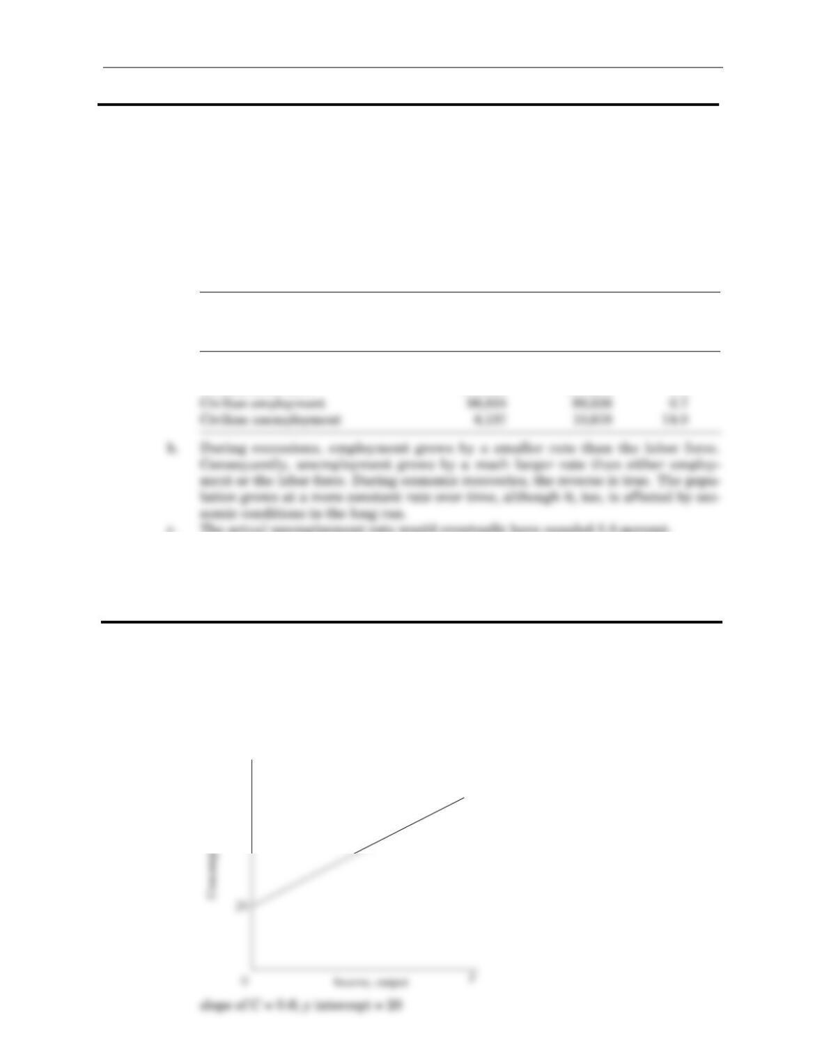
4. a. 0.75
b. Graph for Problem 4(b)
Chapter 9Introduction to Economic Fluctuations 211
CHAPTER 9Introduction to Economic Fluctuations
CHAPTER 10 Aggregate Demand I
C
C


