1
CHAPTER 1
Economic Models
A. Summary
This chapter provides an introduction to the book by showing why economists
use simplified models. The chapter begins with a few definitions of economics
B. Lecture and Discussion Suggestions
We have found that a useful way to start the course is with one (or perhaps two)
lectures on the historical development of microeconomics together with some
current examples. For example, many students find economic applications to the
C. Glossary Entries in the Chapter
• Diminishing Returns
• Economics
• Equilibrium Price
Chapter 1: Economic Models
2
APPENDIX TO CHAPTER 1
Mathematics Used in
Microeconomics
A. Summary
This appendix provides a review of basic algebra with a specific focus on the
graphical tools that students will encounter later in the text. The coverage of
linear and quadratic equations here is quite standard and should be familiar to
students. Two concepts that will be new to some students are graphing con-
tour lines and simultaneous equations. The discussion of contour lines seeks
to introduce students to the indifference curve concept through the contour
map analogy. Although students may not have graphed such a family of
for both variables is particularly instructive in that regard. In that regard, some
material at the end of the appendix makes the distinction between endoge-
nous and exogenous variables – a distinction that many students stumble
B. Lecture and Discussion Suggestions
Since much of the material in this appendix is self-explanatory, most instruc-
tors may prefer to skip any lecture on this topic. For those who feel a lecture
C. Glossary Entries in the Chapter
• Average Effect
• Contour Lines
Chapter 1: Economic Models
3
• Independent Variable
• Intercept
SOLUTIONS TO CHAPTER 1 PROBLEMS
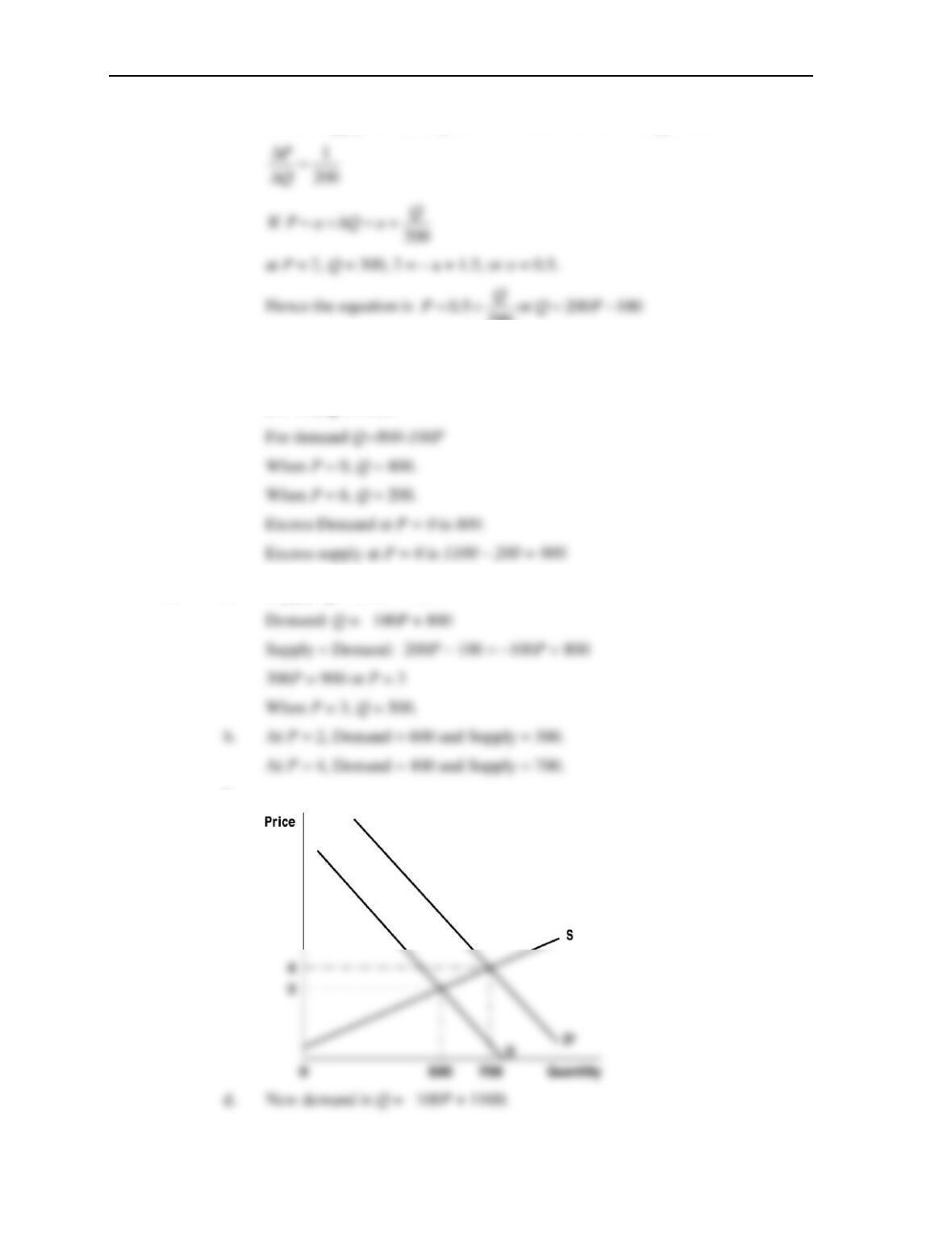
1.1 a.
Chapter 1: Economic Models
4
For the supply curve, the points also seem to be on a straight line:
200
c,d For supply Q = 200P – 100
If P = 0, Q = –100 = 0 (since negative supply is impossible).
If P = 6, Q = 1100.
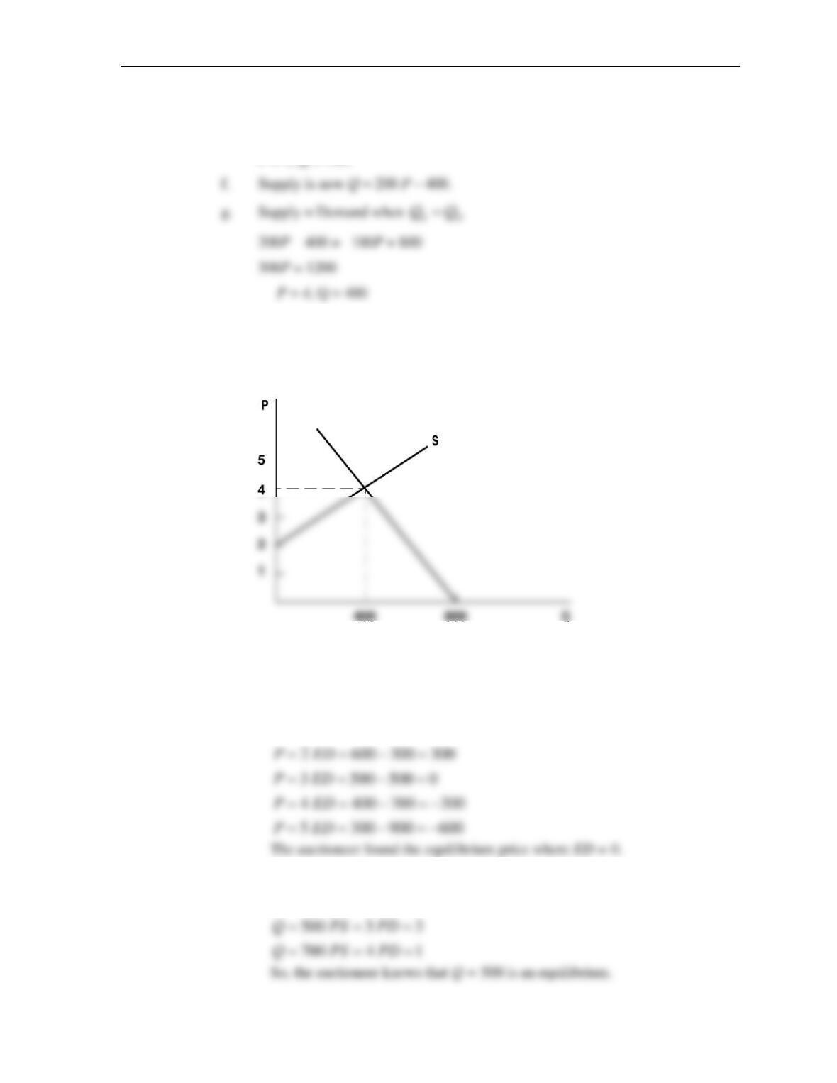
1.2 a. Supply: Q = 200P – 100
c.
Chapter 1: Economic Models
5
e. Supply = Demand: 200P – 100 = –100P + 1100.
300 P = 1200
P = 4, Q = 700.
h. At P = 3,
200, 500==
SD
QQ
; this is not an equilibrium price. Participants
would know this is not an equilibrium price because there would be a shortage
of orange juice.
i.
1.3
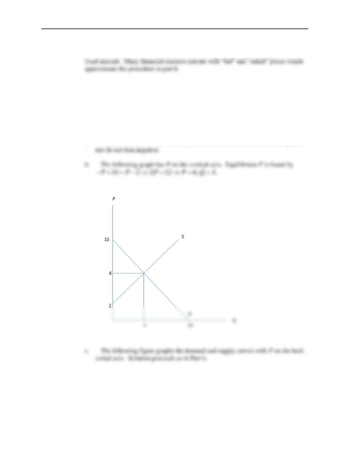
a. Excess Demand is the following at the various prices
1 700 100 600
P ED
= = − =
b. Here is the information the auctioneer gathers from calling quantities:
300 2 5
Q PS PD
= = =
Chapter 1: Economic Models
6
c. Many callout auctions operate this way – though usually quantity supplied is a
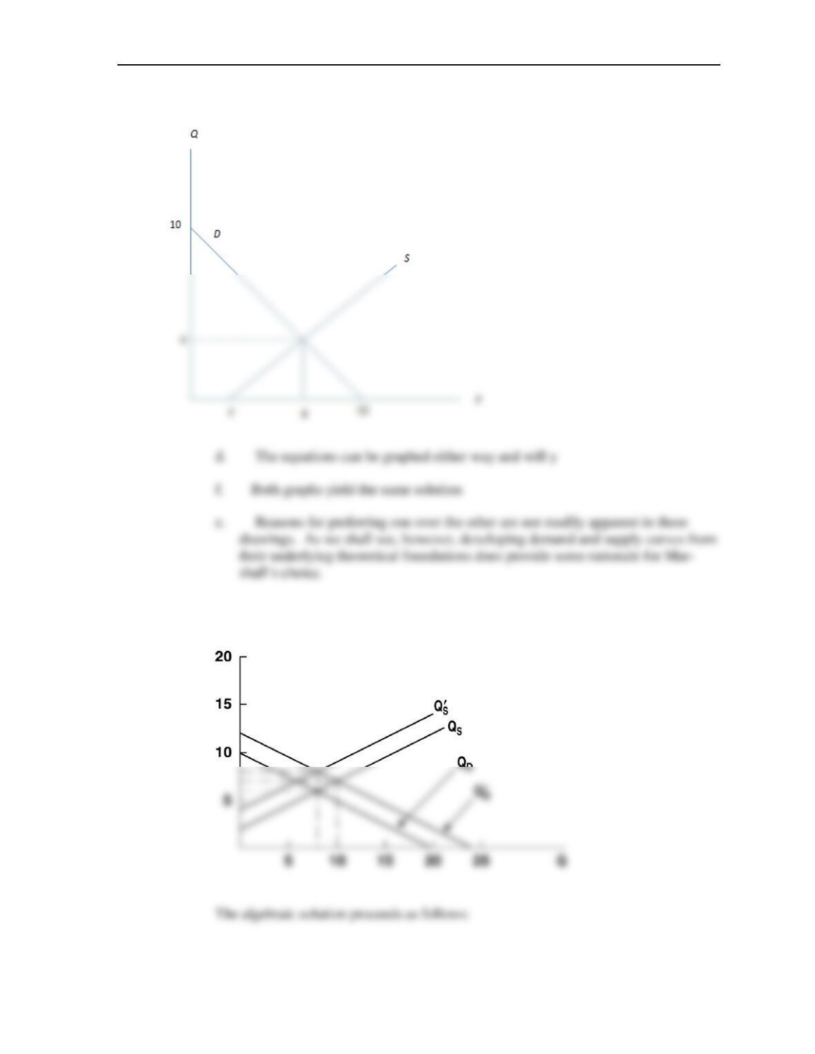
1.4 The complaint is essentially correct – in many economic models price is the inde-
pendent variable and quantity is the dependent variable. Marshall originally chose
this approach because he found it easier to draw cost curves (an essential element of
supply theory) with quantity on the horizontal axis. In that case, quantity can legiti-
mately be treated as the independent variable.
a. The restrictions on P are necessary with linear functions to ensure that quanti-
Chapter 1: Economic Models
7
1.5
a.
Chapter 1: Economic Models
8
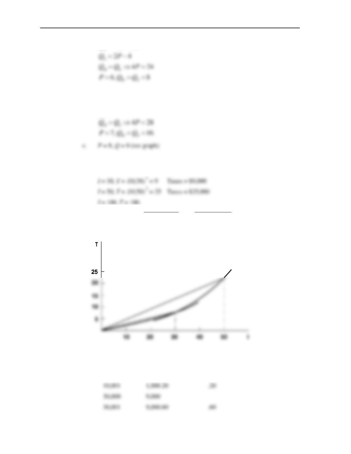
2 20
D
QP
= − +
b.
2 24
D
QP
= − +
1.6 a. T = .01 I 2
I = 10, T = .01(10) 2 = 1 Taxes = $1,000
b. Average Rate Marginal Rate
I = 10,000 10% 20%
I = 30,000 30% 60%
I = 50,000 50% 100%
c.
I T Marginal Tax Rate
10,000 1,000
Chapter 1: Economic Models
9
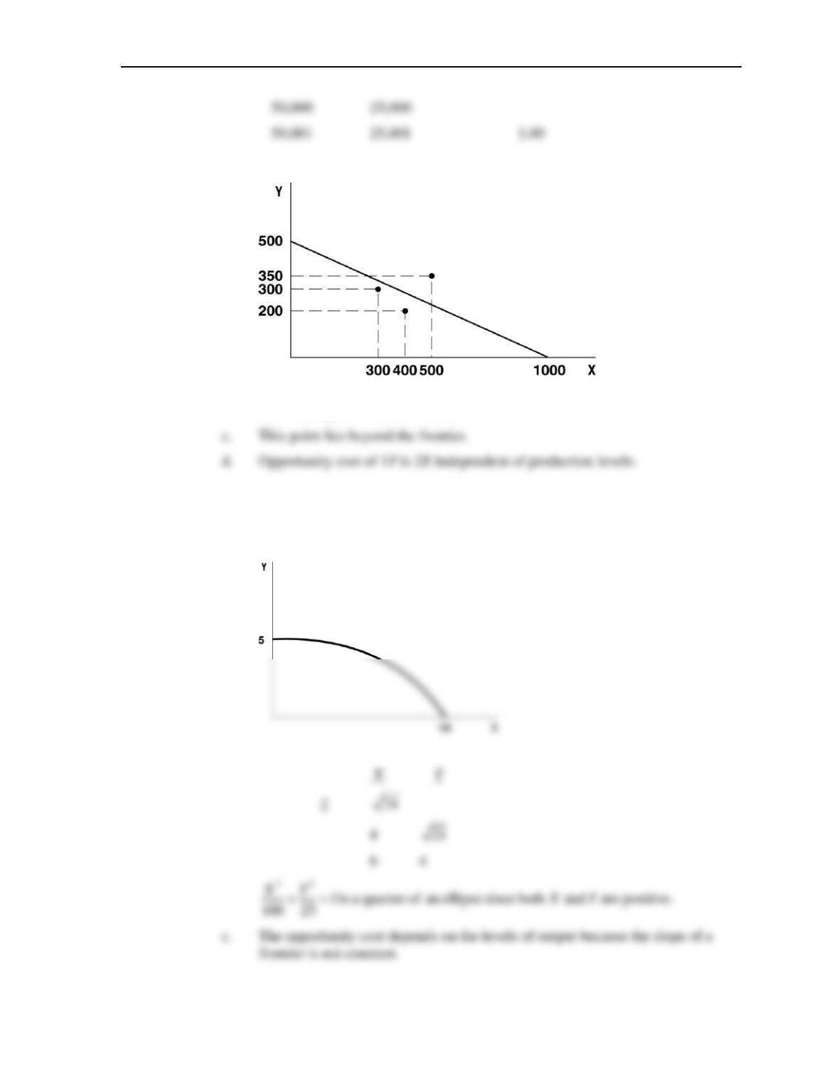
1.7 a.
b. Both these points lie below the frontier.
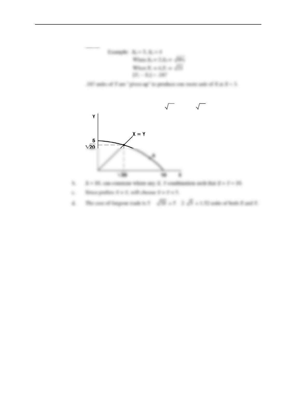
1.8 a. If Y = 0, X = 10
If X= 0, Y = 5
b.
Chapter 1: Economic Models
10
d. The opportunity cost of X is the change in Y when one more unit of X is pro-
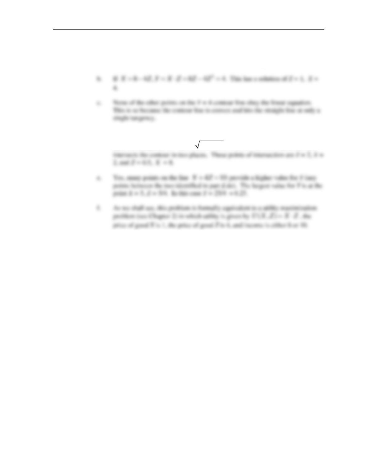
1.9 a. X2 + 4Y2 = 100
If X = Y, then 5X2 = 100 and X =
20
and Y =
20
.
Chapter 1: Economic Models
11
1.10 This problem provides practice with contour lines.
a. If
Y X Z=
the Y = 4 is the same line as “Y = 2” in Figure 1A.5.
d. If
22
10 4 , 10 4 4 or 4 10 4 0X Z Y Z Z Z Z= − = − = − + =
. Using the quad-
ratic formula yields
(10 100 64) / 8 or 2, 0.5ZZ= − =
. Hence the line