
Chapter 1
Econometrics
There are no exercises or applications in Chapter 1.

Chapter 2
The Linear Regression Model
There are no exercises or applications in Chapter 2.
Chapter 3
Least Squares
◼ Exercises
1. Let
1
1
.
1n
x
x
=
X
a. The normal equations are given by (3-12),
X e 0=
(we drop the minus sign), hence for each
c. We know that
n
e
=
and
n
xe
=
It follows then that
n
x x e
− =
d. The first derivative vector of ee is −2Xe. (The normal equations.) The second derivative matrix is
2. Write c as b + (c − b). Then, the sum of squared residuals based on c is
(y − Xc) (y − Xc) = [y − X(b + (c − b))] [y − X(b + (c − b))]
3. In the regression of y on i and X, the coefficients on X are b = (XMX)−1XMy. M = I − i(ii)−1i
is the matrix which transforms observations into deviations from their column means. Since M0 is
4. What is the result of the matrix product M1M where M1 is defined in (3-19) and M is defined in (3-14)?
5. The original X matrix has n rows. We add an additional row, xs. The new y vector likewise has an
additional element. Thus,
and .
nn
n,s n,s
ss
y
==
Xy
Xy
x
The new coefficient vector is
bn −
1
1
1()
1 ( ) n n s s n
−
−
+X X x x b
x X X x
+
1
()
nn
−
XX
xsys
11
1
1( ) ( )
1 ( ) n n s s n n
−−
−
−
+X X x x X X
x X X x
xs ys
6. Define the data matrix as follows:
1 1 2
, and .
1 0 1 1
o
m
y
= = = =
y
i x 0 0
X X X X y
6 Greene • Econometric Analysis, Seventh Edition
7. For convenience, reorder the variables so that X = [i, Pd, Pn, Ps, Y]. The three dependent variables are Ed,
En, and Es, and Y = Ed + En + Es. The coefficient vectors are
bd = (XX)−1XEd,
8. Let
2
K
R
denote the adjusted R2 in the full regression on K variables including xk, and let
2
1
R
denote the
adjusted R2 in the short regression on K-1 variables when xk is omitted. Let
2
K
R
and
2
1
R
denote their
unadjusted counterparts. Then,
Then,
2
K
R
= 1 − [(n − 1)/(n − K)](1 −
2)
K
R
9. This R2 must be lower. The sum of squares associated with the coefficient vector which omits the
10. We use the notations ‘Var[.]’ and ‘Cov[.]’ to indicate the sample variances and covariances. Our
information is
Var[N] = 1, Var[D] = 1, Var[Y] = 1.
Since C = N + D, Var[C] = Var[N] + Var[D] + 2Cov[N, D] = 2(1 + Cov[N, D]).
From the regressions, we have
11. The relevant submatrices to be used in the calculations are
Investment Constant GNP Interest
Investment * 3.0500 3.9926 23.521
The inverse of the lower right 3 3 block is (XX)−1,
7.5874
12. The results cannot be correct. Since log S/N = log S/Y + log Y/N by simple, exact algebra, the same result
must apply to the least squares regression results. That means that the second equation estimated must equal
8 Greene • Econometric Analysis, Seventh Edition
Application
?=======================================================================
? Chapter 3 Application 1
?=======================================================================
Read $
(Data appear in the text.)
Namelist ; X1 = one,educ,exp,ability$
Namelist ; X2 = mothered,fathered,sibs$
?=======================================================================
? a.
?=======================================================================
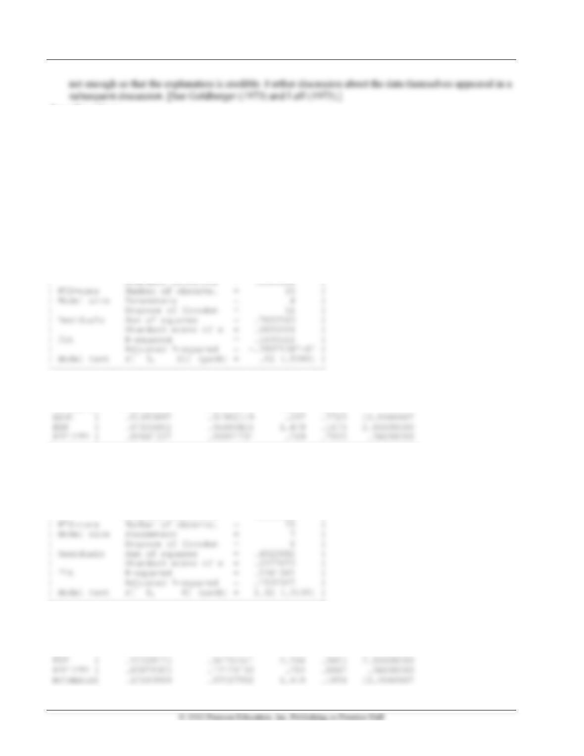
Regress ; Lhs = wage ; Rhs = x1$
+—————————————————-+
| Ordinary least squares regression |
| LHS=WAGE Mean = 2.059333 |
+—————————————————-+
+——–+————–+—————-+——–+——–+———-+
|Variable| Coefficient | Standard Error |t-ratio |P[|T|>t]| Mean of X|
+——–+————–+—————-+——–+——–+———-+
Constant| 1.66364000 .61855318 2.690 .0210
?=======================================================================
? b.
?=======================================================================
Regress ; Lhs = wage ; Rhs = x1,x2$
+—————————————————-+
| Ordinary least squares regression |
| LHS=WAGE Mean = 2.059333 |
| Standard deviation = .2583869 |
+—————————————————-+
+——–+————–+—————-+——–+——–+———-+
|Variable| Coefficient | Standard Error |t-ratio |P[|T|>t]| Mean of X|
+——–+————–+—————-+——–+——–+———-+
Constant| .04899633 .94880761 .052 .9601
EDUC | .02582213 .04468592 .578 .5793 12.8666667

Chapter 3 Least Squares 9
10 Greene • Econometric Analysis, Seventh Edition
?=======================================================================
? c.
?=======================================================================
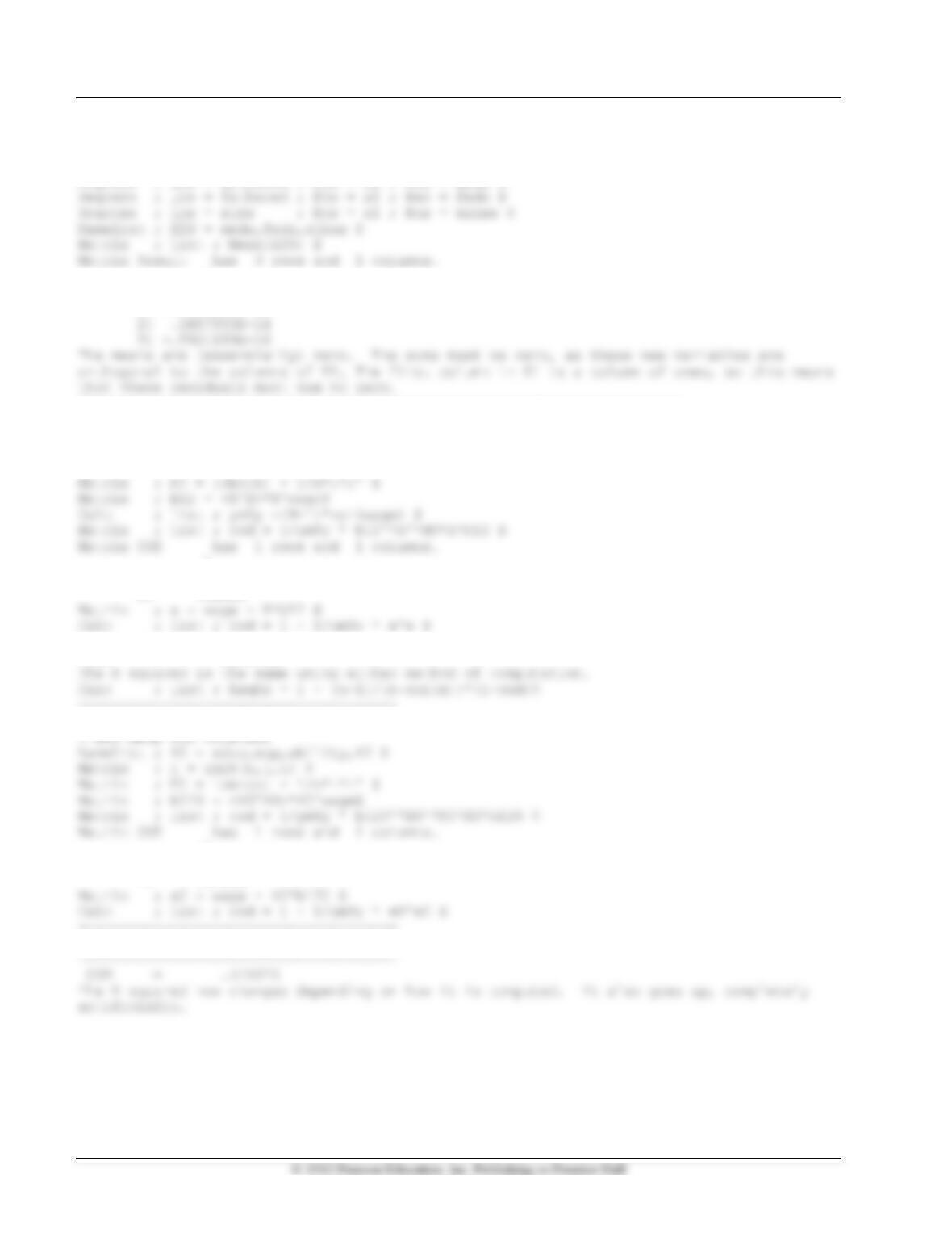
Regress ; Lhs = mothered ; Rhs = x1 ; Res = meds $
1
+————–
1| -.1184238D-14
?=======================================================================
? d.
?=======================================================================
Namelist ; X = X1,X2 $
Matrix ; i = init(n,1,1) $
1
+————–
1| .51613
+————————————+
COD = .516134
+————————————+
RSQAD = .153235
1
+————–
1| .52953
+————————————+
| Listed Calculator Results |
Chapter 3 Least Squares 11
?=======================================================================
? e.
?=======================================================================
? f.
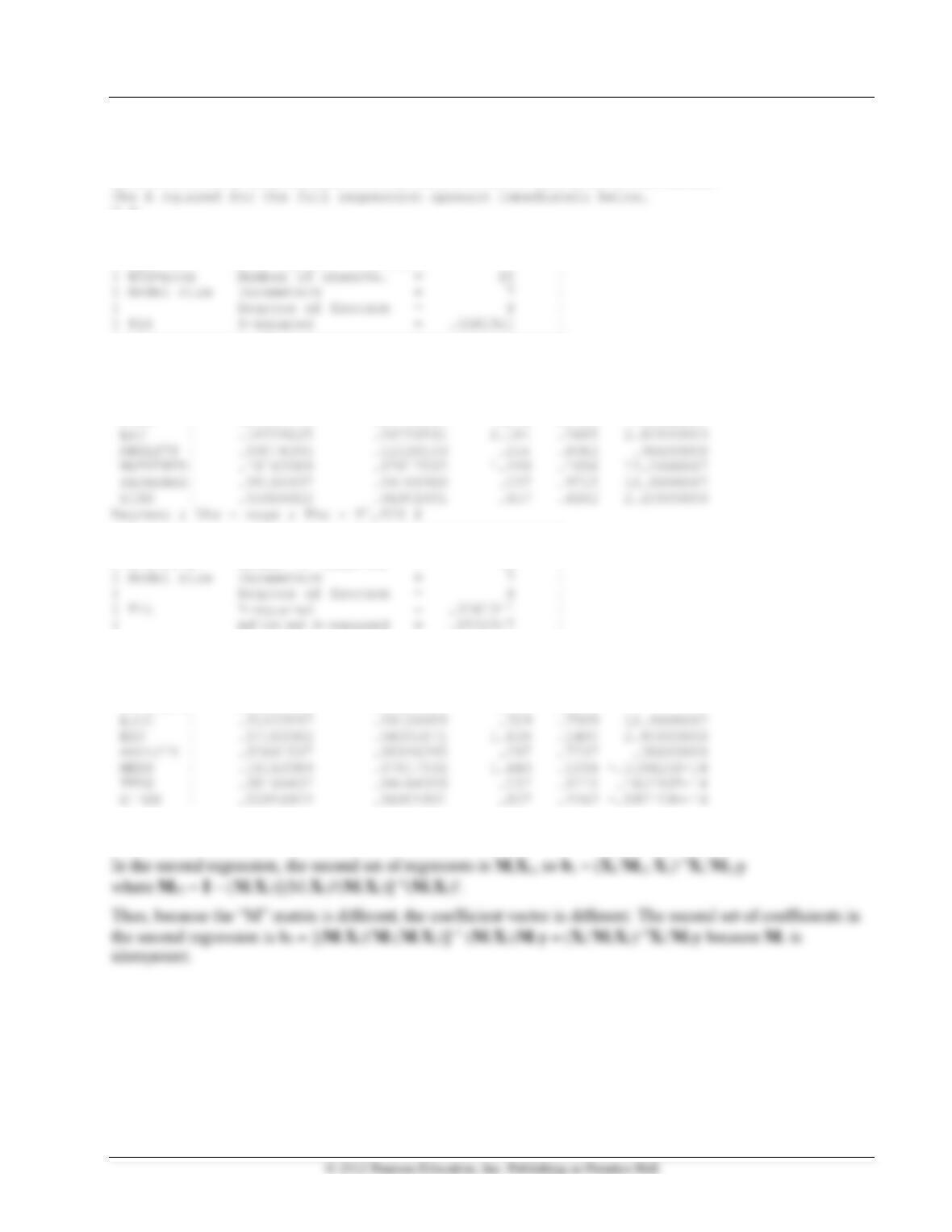
Regress ; Lhs = wage ; Rhs = X1,X2 $
+—————————————————-+
| Ordinary least squares regression |
+—————————————————-+
+——–+————–+—————-+——–+——–+———-+
|Variable| Coefficient | Standard Error |t-ratio |P[|T|>t]| Mean of X|
+——–+————–+—————-+——–+——–+———-+
Constant| .04899633 .94880761 .052 .9601
EDUC | .02582213 .04468592 .578 .5793 12.8666667
+—————————————————-+
| Ordinary least squares regression |
| WTS=none Number of observs. = 15 |
+—————————————————-+
+——–+————–+—————-+——–+——–+———-+
|Variable| Coefficient | Standard Error |t-ratio |P[|T|>t]| Mean of X|
+——–+————–+—————-+——–+——–+———-+
Constant| 1.66364000 .55830716 2.980 .0176
In the first set of results, the first coefficient vector is b1 = (X1M2X1)−1X1M2y and b2 = (X2M1X2)−1X2M1y.