Appendix E
Computation and Optimization
◼ Exercises
1. Show how to maximize the function
2
( ) /2
1
() 2
c
fe
− −
=
with respect to for a constant, c, using Newton’s method. Show that maximizing logf() leads to the
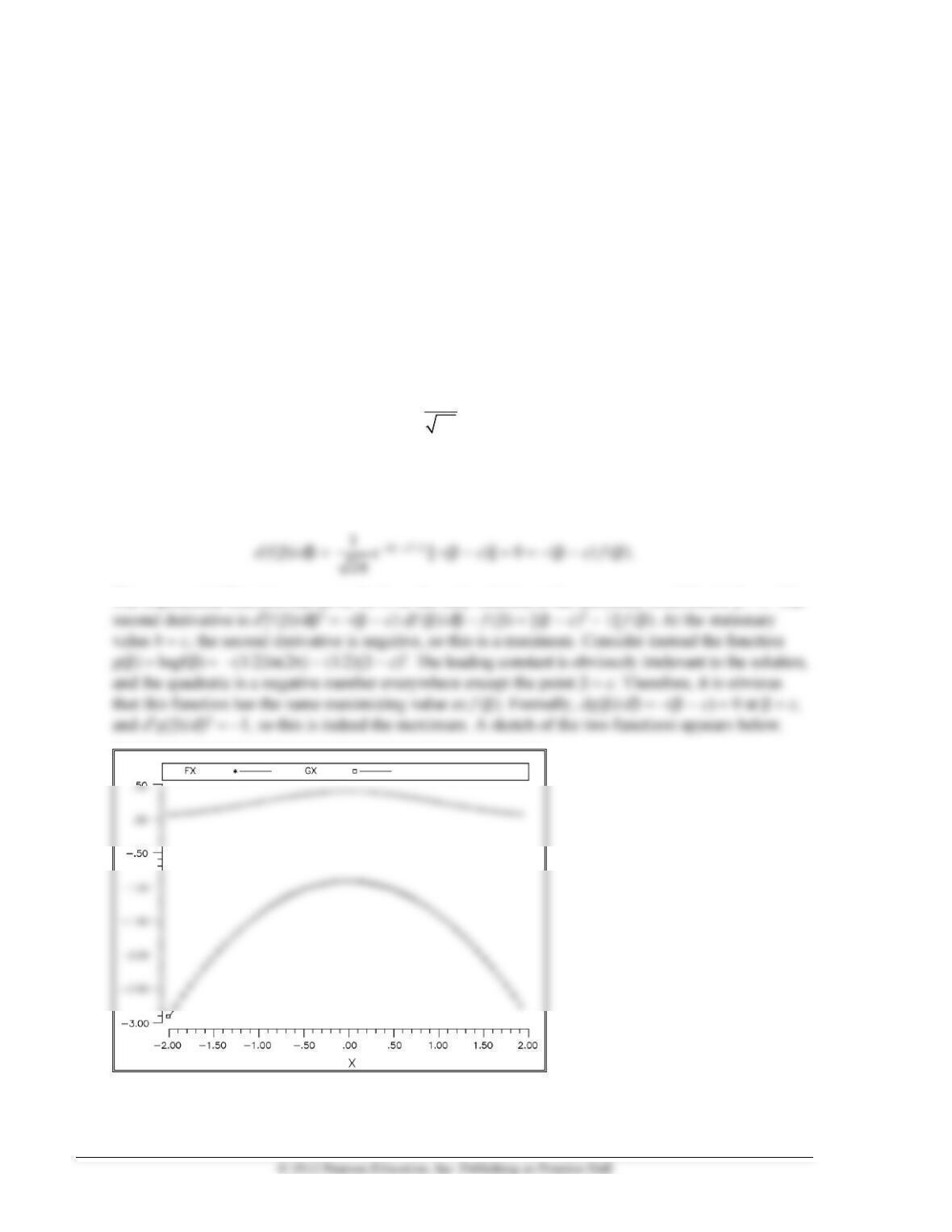
same solution. Plot f() and logf().
The necessary condition for maximizing f() is
The exponential function can never be 0, so the only solution to the necessary condition is = c. The
Note that the transformed function is concave everywhere while the original function has inflection points.
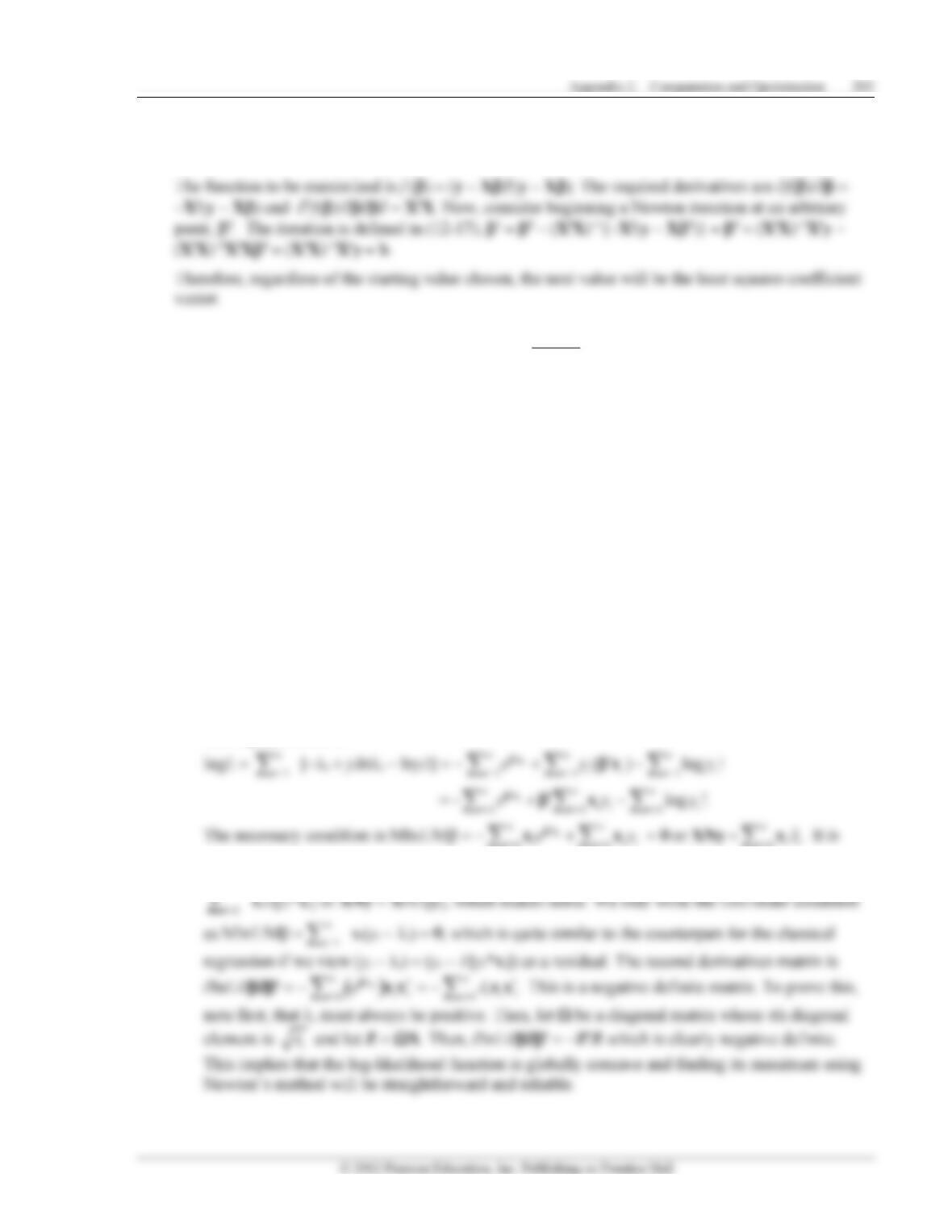
2. Prove that Newton’s method for minimizing the sum of squared residuals in the linear regression
model will converge to the minimum in one iteration.
3. For the Poisson regression model, Prob[Yi = yi|xi] =
!
ii
y
i
i
e
y
−
where i =
.
i
e
x
The log-likelihood
function is ln L =
1
n
i=
logProb[Yi = yi|xi].
(a) Insert the expression for i to obtain the log-likelihood function in terms of the observed data.
(b) Derive the first-order conditions for maximizing this function with respect to .
(c) Derive the second derivatives matrix of this criterion function with respect to . Is this matrix
negative definite?
(d) Define the computations for using Newton’s method to obtain estimates of the unknown parameters.
(e) Write out the full set of steps in an algorithm for obtaining the estimates of the parameters of this
model. Include in your algorithm a test for convergence of the estimates based on Belsley’s
suggested criterion.
(f) How would you obtain starting values for your iterations?
(g) The following data are generated by the Poisson regression model with log = + x.
y 6 7 4 10 10 6 4 7 2 3 6 5 3 3 4
x 1.5 1.8 1.8 2.0 1.3 1.6 1.2 1.9 1.8 1.0 1.4 0.5 0.8 1.1 0.7
Use your results from parts (a)−(f) to compute the maximum likelihood estimates of and .
Also obtain estimates of the asymptotic covariance matrix of your estimates.
The log likelihood is
11
ii
==
1.
i
=
useful to note, since E[yi*xi] = i = eNxi, the first-order condition is equivalent to
1
n
ii
iy
=
x
=
n
n
(1) Obtain starting values for the parameters. Because the log-likelihood function is globally
concave, it will usually not matter what values are used. Most applications simply use 0.
1
−
(3) Each time we compute
1
ˆ,
t+
we should check for convergence. Some possibilities are
(a) Gradient: Are the elements of lnL/ small?
(b) Change: Is
1
ˆˆ
tt+−
small?
(4) When convergence has been achieved, the asymptotic covariance matrix for the estimates is
estimated with the inverse matrix used in the iterations.
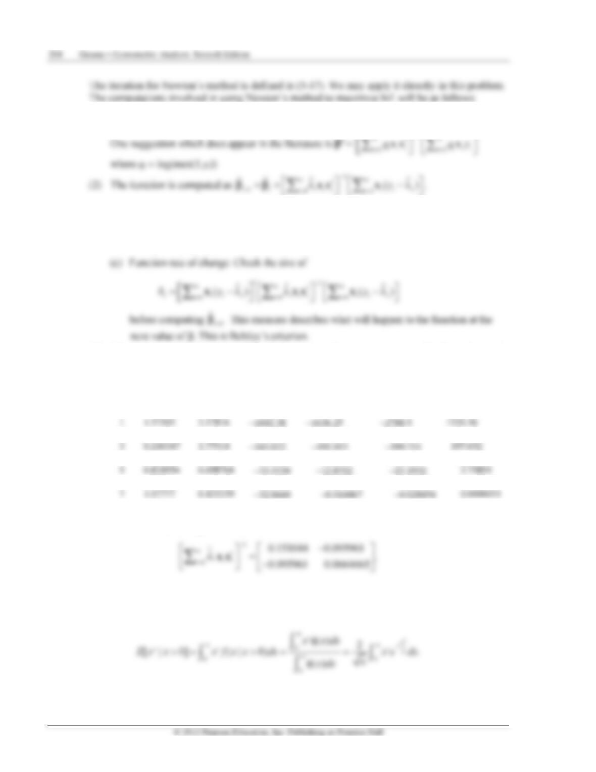
Using the data given in the problem, the results of the above computations are
Iter.
lnL
lnL/
lnL/
Change
0
0
0
−102.387
65.0
95.1
296.261
1
1.37105
2.17816
1526.36
2
0.619874
2.05865
−461.989
−581.966
−996.711
516.92
3
0.210347
1.77914
−141.022
−195.953
−399.751
197.652
4
0.351893
1.26291
−51.2989
−57.9294
−102.847
30.616
5
0.824956
0.698768
−33.5530
−12.8702
2.75855
6
1.05288
0.453352
−32.0824
−1.28785
−2.29289
0.032399
7
1.07777
0.425239
−32.0660
−0.016067
−0.028454
0.0000051
8
1.07808
0.424890
−32.0660
0
0
0
At the final values, the negative inverse of the second derivatives matrix is
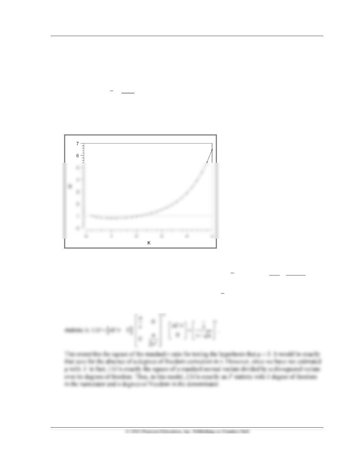
4. Use the Monte Carlo integration to plot the function g(r) = E[xr*x > 0] for the standard normal distribution.
The expected value from the truncated normal distribution is
Appendix E Computation and Optimization 205
To evaluate this expectation, we first sampled 1000 observations from the truncated standard normal
distribution using (5-1). For the standard normal distribution, = 0, = 1, PL = ((0 − 0)/1) = 2, and PU
= ((+ 4 − 0)/1) = 1. Therefore, the draws are obtained by transforming draws from U(0,1) (denoted Fi) to
xi = [2(1 + Fi)]. Since 0 < Fi < 1, the argument in brackets must be greater than 2, so xi > 0, which is to
be expected. Using the same 1000 draws each time (so as to obtain smoothness in the figure), we then
plot the values of
1000
1
1,
1000
r
ri
i
xx
=
=
r = 0, 0.2, 0.4, 0.6, …, 5.0. As an additional experiment, we
generated a second sample of 1000 by drawing observations from the standard normal distribution and
discarding them and redrawing if they were not positive. The means and standard deviations of the two
samples were (0.8097, 0.6170) for the first and (0.8059, 0.6170) for the second. Drawing the second
sample takes approximately twice as long as the second. Why?
5. For the model in Example 5.10, derive the LM statistic for the test of the hypothesis that = 0.
The derivatives of the log likelihood with = 0 imposed are g =
2
/nx
and
2
2
1
24
.
22
n
i
ix
n
g=
−
=+
The estimator for 2 will be obtained by equating the second of these to 0, which will give (of course),
v = xx/n. The terms in the Hessian are H = −n/2,
2
4
/H nx
= −
, and
22
H =
n/(24) − xx/6. At
the MLE,
2
g
= 0, exactly. The off-diagonal term in the expected Hessian is also 0. Therefore, the LM
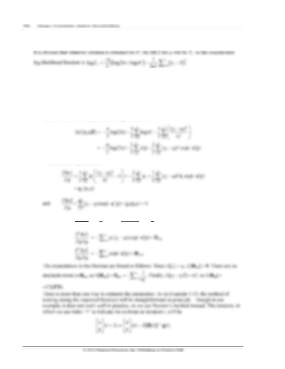
6. In Example 5.10, what is the concentrated over log-likelihood function?
7. In Example E.13, suppose that E[yi] = , for a nonzero mean.
(a) Extend the model to include this new parameter. What are the new log likelihood, likelihood
equation, Hessian, and expected Hessian?
(b) How are the iterations carried out to estimate the full set of parameters?
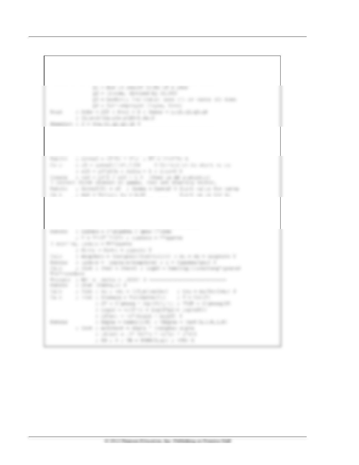
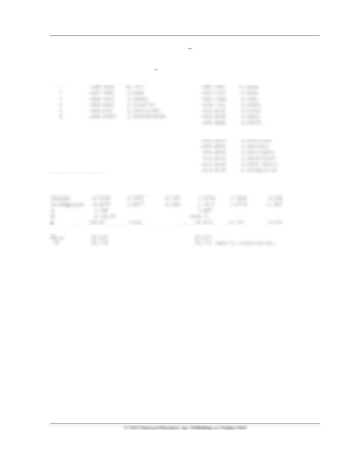
(c) Show how the LIMDEP program should be modified to include estimation of .
(d) Using the same data set, estimate the full set of parameters.
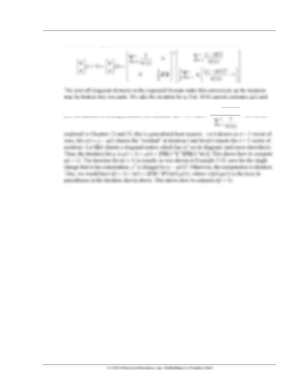
If yi has a nonzero mean, , then the log likelihood is
The likelihood equations are
The Hessian is
2ln L
=
2
2
1
()
1
2
n
i
ii
ii
y
=
−
−
zz
=
1
1( exp( )
2
n
i i i i
i
y
=
− − −
2
) z z z
= H
Appendix E Computation and Optimization 207
If we insert the expected Hessians and first derivatives in this iteration, we obtain
12
()
() .
ni
i
i
yt
t
=
−
208 Greene • Econometric Analysis, Seventh Edition
/*================================================================
Program Code for Estimation of Harvey’s Model
The data set for this model is 100 observations from Greene (1992)
Variables are: Y = Average monthly credit card expenditure
================================================================
Step 1 is to get the starting values and set some values for the
iterations− iter=iteration counter, delta=value for convergence.
*/
Create ; y0 = y – Xbr(y) ; ui = log(y0^2) $
Procedure −−−−−−−−−−[This does the iterations]−−−−−−−−−−−−−−−−−−−−
Create ; vari = exp(Z’Gamma) ; ei = y−mu ; varinv=1/vari
; hi = ei^2 / vari
; gigamma = .5*(hi − 1); gimu = ei/vari
; logli = −.5*(log(2*pi) + log(vari) + hi) $
Appendix E Computation and Optimization 209
In the Example in the text, was constrained to equal
.y
In the program, is allowed to be a free
parameter. The comparison of the two sets of results appears below.
(Constrained model, =
y
) (Unconstrained model)
Iteration log likelihood log likelihood
−679.4568 0.0101793
−679.4542 0.00364255
Estimated Paramaters
Variable Estimate Std Error t−ratio Estimate Std Error t−ratio
Age 0.013042 0.02310 0.565 −0.0134 0.0244 −0.550
Income 0.6432 0.120001 5.360 0.9953 0.1375 7.236
Tests of the joint hypothesis that all slope coefficients are zero: