Appendix C
Estimation and Inference
◼ Exercises
1. The following sample is drawn from a normal distribution with mean and standard deviation :
x = 1.3, 2.1, 0.4, 1.3, 0.5, 0.2, 1.8, 2.5, 1.9, 3.2.
Compute the mean, median, variance, and standard deviation of the sample.
2. Using the data in the previous exercise, test the following hypotheses:
(a) > 2.
(b) < 0.7.
(c) 2 = 0.5.
(d) Using a likelihood ratio test, test the following hypothesis = 1.8, 2 = 0.8.
(a) We would reject the hypothesis if 1.52 is too small relative to the hypothesized value of 2.
(b) We would reject the hypothesis if 1.52 is excessively large relative to the hypothesized mean
(c) The statistic (n −1)s2/2 is distributed as 2 with 9 degrees of freedom. This is 9(0.94)/0.5 =
Appendix C Estimation and Inference 189
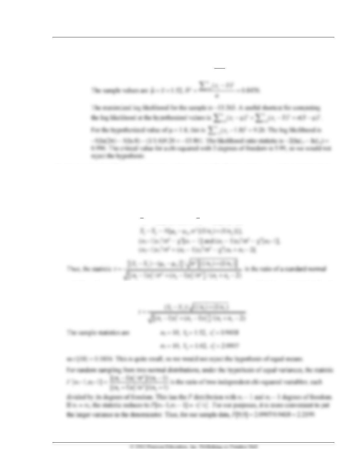
(d) The log likelihood for a sample from a normal distribution is
22
1
2
1
ln ( /2)ln(2 ) ( /2)ln ( ) .
2
n
i
i
L n n x
=
= − − − −
3. Suppose that the following sample is drawn from a normal distribution with mean and standard deviation
: y = 3.1, −0.1, 0.3, 1.4, 2.9, 0.3, 2.2, 1.5, 4.2, 0.4. Test the hypothesis that the mean of the distribution
which produced these data is the same as that which produced the data in Exercise 1. Test the hypothesis
assuming that the variances are the same. Test the hypothesis that the variances are the same using an
F test and using a likelihood ratio test. (Do not assume that the means are the same.)
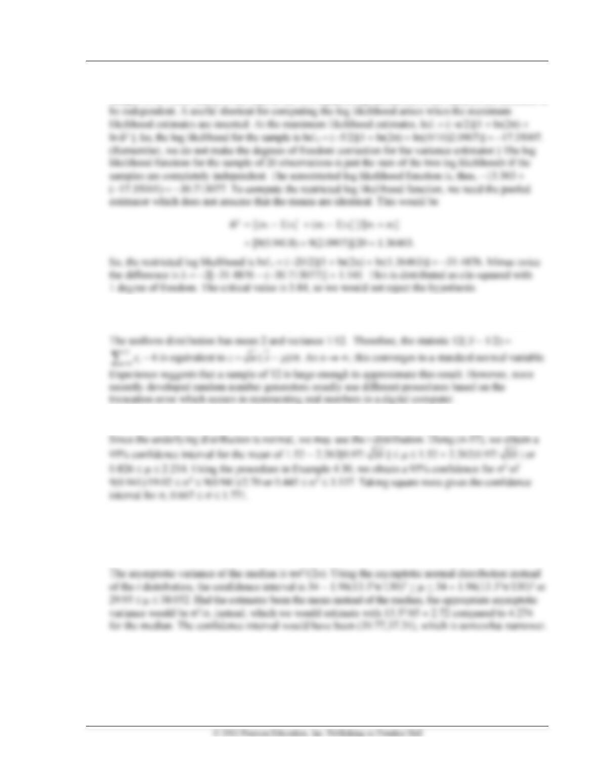
If the variances are the same,
2
1 1 1
~ [ , / ]x N n
and
2
2 2 2
~ [ , / ],x N n
variable to the square root of a chi-squared variable divided by its degrees of freedom, which is distributed
as t with n1 + n2 − 2 degrees of freedom. Under the hypothesis that the means are equal, the statistic is

190 Greene • Econometric Analysis, Seventh Edition
Appendix C Estimation and Inference 191
The likelihood ratio test is based on the test statistic = −2(lnLr − lnLu). The log likelihood for the joint
sample of 20 observations is the sum of the two separate log likelihoods if the samples are assumed to
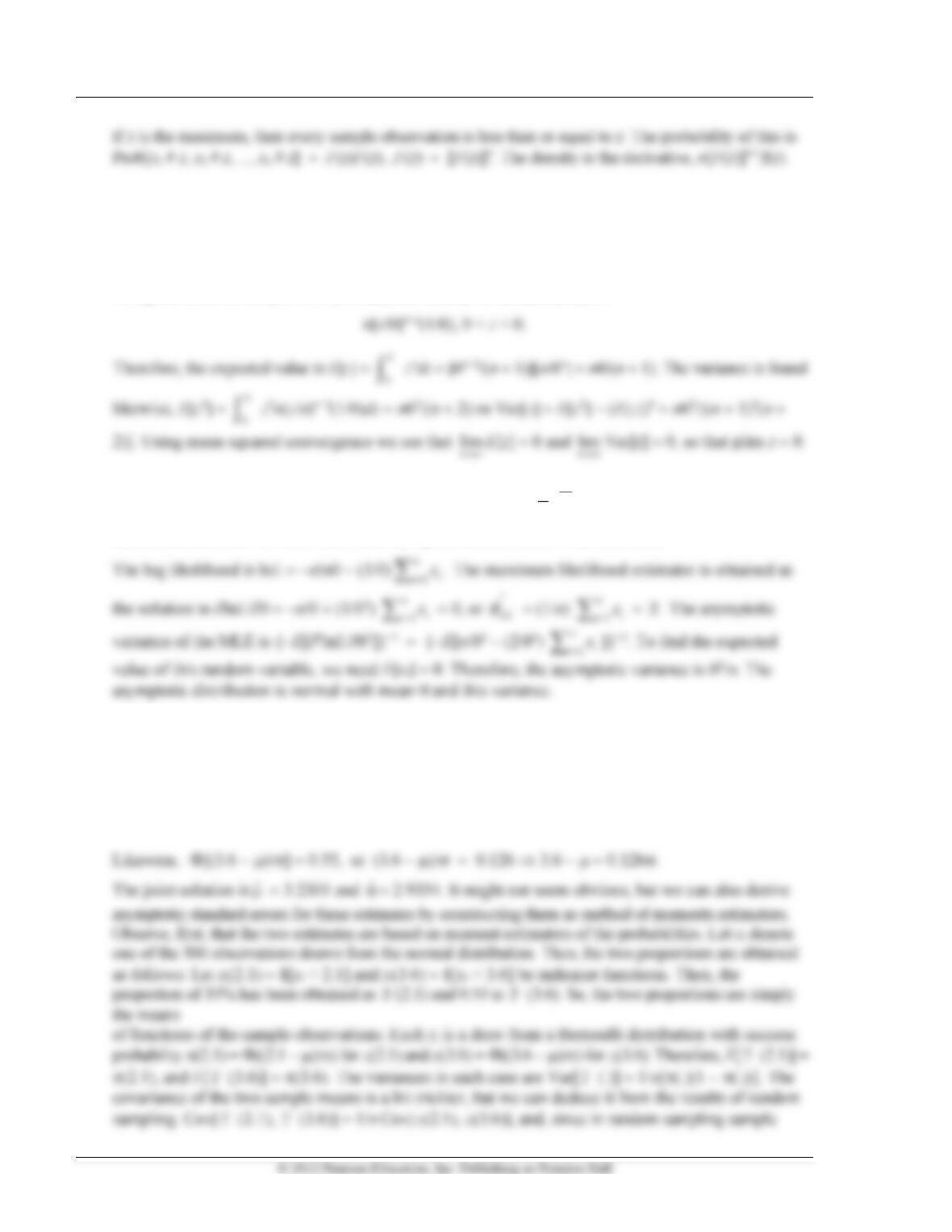
4. A common method of simulating random draws from the standard normal distribution is to compute
the sum of 12 draws from the uniform [0,1] distribution and subtract 6. Can you justify this procedure?
5. Using the data in Exercise 1, form confidence intervals for the mean and standard deviation.
6. Based on a sample of 65 observations from a normal distribution, you obtain a median of 34 and a
standard deviation of 13.3. Form a confidence interval for the mean. (Hint: Use the asymptotic
distribution. See Example 4.15.) Compare your confidence interval to the one you would have
obtained had the estimate of 34 been the sample mean instead of the sample median.
7. The random variable x has a continuous distribution f (x) and cumulative distribution function F(x). What
is the probability distribution of the sample maximum? (Hint: In a random sample of n observations, x1,
x2, …, xn, if z is the maximum, then every observation in the sample is less than or equal to z. Use the CDF.)
192 Greene • Econometric Analysis, Seventh Edition
8. Assume the distribution of x is f (x) = 1/, 0 x . In random sampling from this distribution, prove
that the sample maximum is a consistent estimator of . Note: You can prove that the maximum is the
maximum likelihood estimator of . But, the usual properties do not apply here. Why not? (Hint:
Attempt to verify that the expected first derivative of the log likelihood with respect to is zero.)
Using the result of the previous problem, the density of the maximum is
9. In random sampling from the exponential distribution, f (x) =
1,
x
e
−
x > 0, > 0, find the maximum
likelihood estimator of and obtain the asymptotic distribution of this estimator.
10. Suppose in a sample of 500 observations from a normal distribution with mean and standard
deviation , you are told that 35% of the observations are less than 2.1 and 55% of the observations
are less than 3.6. Estimate and .
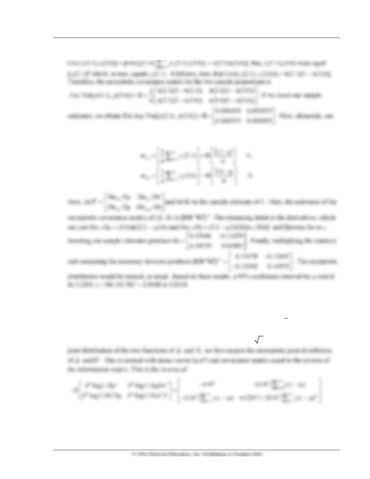
If 35% of the observations are less than 2.1, we would infer that
[(2.1 − )/] = 0.35, or (2.1 − )/ = −0.385 2.1 − = − 0.385.
Appendix C Estimation and Inference 193
moments will converge to their population counterparts,
estimates of and are found as functions of p(2.1) and p(3.6), using the method of moments.
The moment equations are
11. For random sampling from a normal distribution with nonzero mean and standard deviation ,
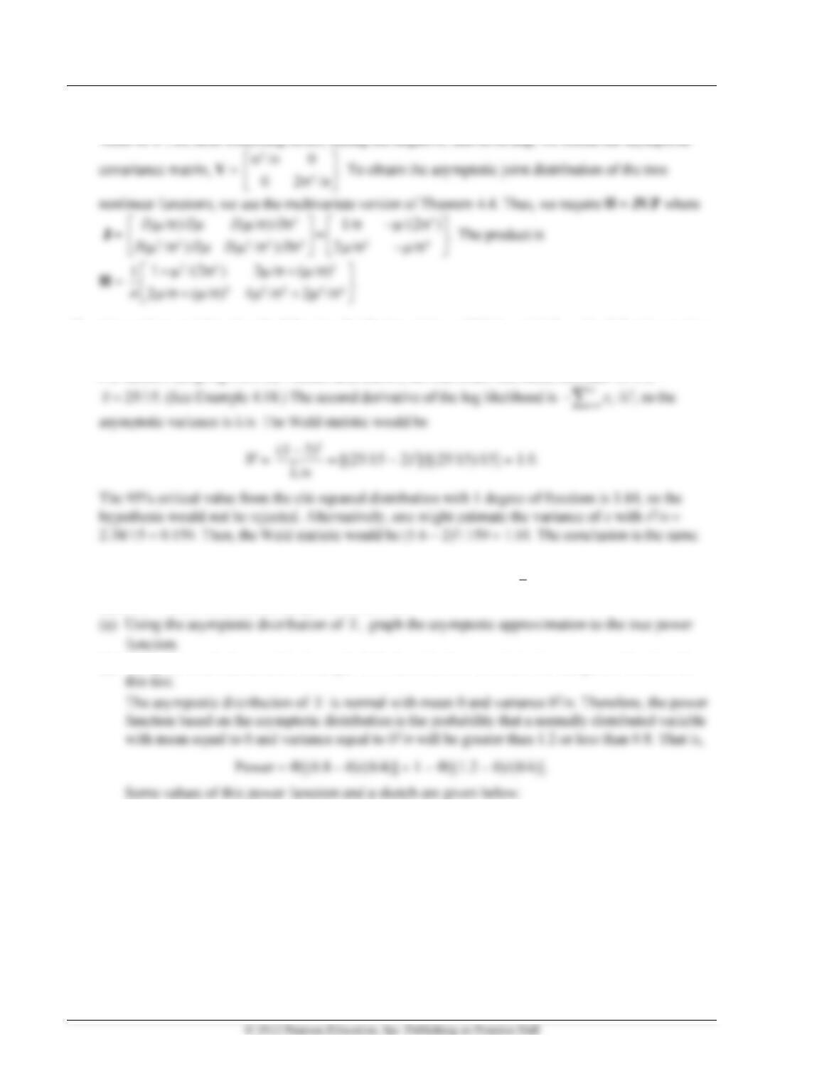
find the asymptotic joint distribution of the maximum likelihood estimators of / and 2/2.
The maximum likelihood estimators,
ˆ
= (1/n)
1
n
i
ix
=
and
2
ˆ
= (1/n)
2
1()
n
i
ixx
=−
were given in
(4-49). By the invariance principle, we know that the maximum likelihood estimators of / and
2/2 are
ˆˆ
/
and
2
ˆˆ
/
and the maximum likelihood estimate of is
ˆ.
To obtain the asymptotic
194 Greene • Econometric Analysis, Seventh Edition
The off-diagonal term has an expected value of 0. Each term in the sum in the lower right has an expected
value of 2, so, after collecting terms, taking the negative, and inverting, we obtain the asymptotic
12. The random variable x has the following distribution: f (x) = e−x/x!, x = 0,1,2,…. The following random
sample is drawn: 1,1,4,2,0,0,3,2,3,5,1,2,1,0,0. Carry out a Wald test of the hypothesis that = 2.
For random sampling from the Poisson distribution, the maximum likelihood estimator of is
13. Based on random sampling of 16 observations from the exponential distribution of Exercise 9, we
wish to test the hypothesis that =1. We will reject the hypothesis if
x
is greater than 1.2 or less
than 0.8. We are interested in the power of this test.
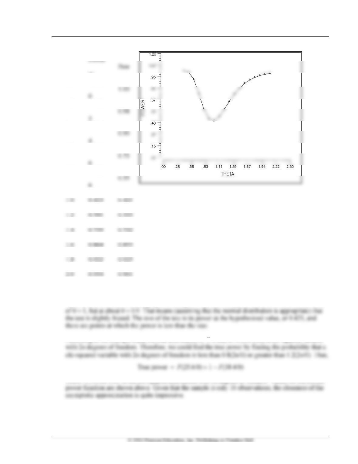
(b) Using the result discussed in Example 4.17, describe how to obtain the true power function for
Appendix C Estimation and Inference 195
Approx. True
er
0.4 1.000
0.5 0.992
0.6 0.908
0.7 0.718
0.8 0.522
0.9 0.420 0.443
1.1 0.496 0.470
1.3 0.685 0.647
1.5 0.819 0.801
1.7 0.897 0.895
1.9 0.940 0.946
2.1 0.963 0.972
Note that the power function does not have the symmetric shape of Figure 4.7 because both the
variance and the mean are changing as changes. Moreover, the power is not the lowest at the value
According to the example cited, the true distribution of
x
is that of /(2n) times a chi-squared variable
where F(.) is the CDF of the chi-squared distribution with 32 degrees of freedom. Values for the correct
196 Greene • Econometric Analysis, Seventh Edition
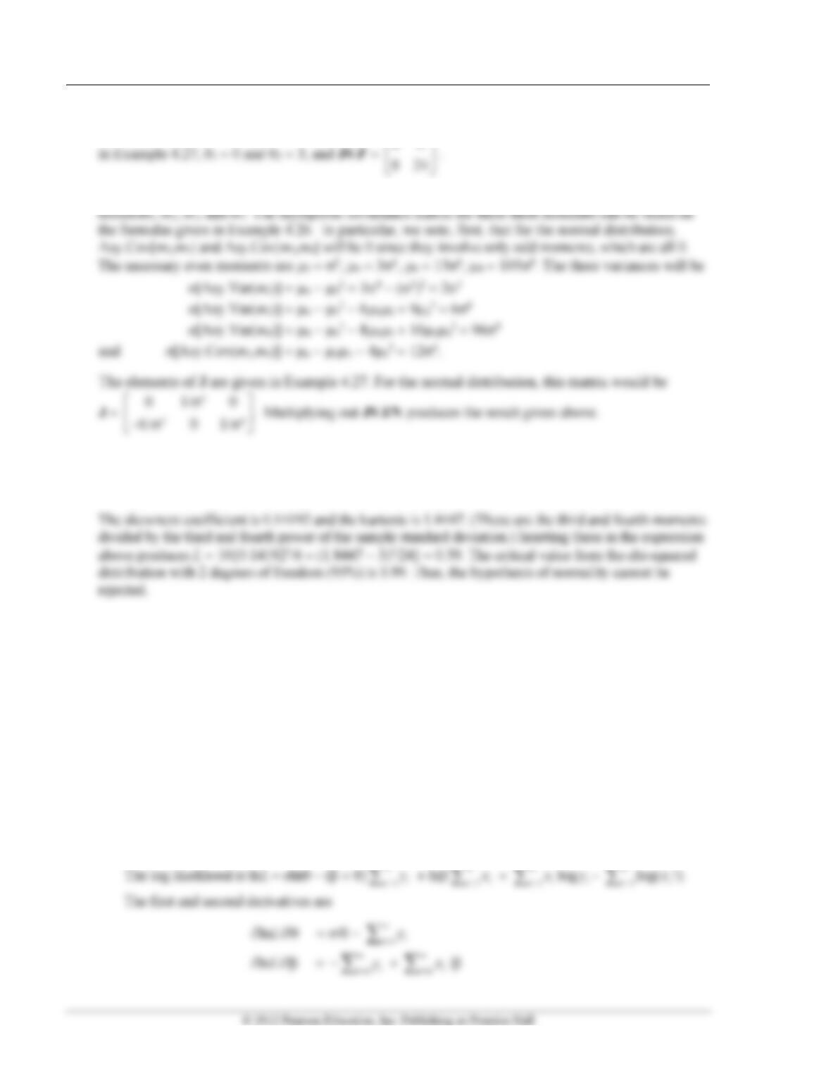
14. For the normal distribution, 2k = 2k(2k)!/(k!2k) and 2k+1 = 0, k = 0,1,…. Use this result to show that
For 1 and 2, just plug in the result above using k = 2, 3, and 4. The example involves three
15. Testing for normality. One method that has been suggested for testing whether the distribution
underlying a sample is normal is to refer the statistic L = n{skewness2/6 + (kurtosis −3)2/24} to the
chi-squared distribution with 2 degrees of freedom. Using the data in Exercise 1, carry out the test.
16. Suppose the joint distribution of the two random variables x and y is
f(x,y) =
()
( ) / !
yx
e y x
− +
, 0, y $ 0, x = 0,1,2,….
(a) Find the maximum likelihood estimators of and and their asymptotic joint distribution.
(b) Find the maximum likelihood estimator of /( + ) and its asymptotic distribution.
(c) Prove that f(x) is of the form f(x) = (1 − )x, x = 0,1,2,….
Then, find the maximum likelihood estimator of and its asymptotic distribution.
(d) Prove that f(y*x) is of the form e−y(y) x/x!. Prove that f(y|x) integrates to 1. Find the maximum
likelihood estimator of and its asymptotic distribution. (Hint: In the conditional distribution, just
carry the xs along as constants.)
(e) Prove that f (y) = e−y then find the maximum likelihood estimator of and its asymptotic variance.
(f) Prove that f (x|y) = e−y (y) x/x!. Based on this distribution, what is the maximum likelihood
estimator of ?
Appendix C Estimation and Inference 197
00
This is x(/x!) times a gamma integral. This is f (x) = x(/x!)[(x + 1)]/( + )x + 1. But, (x + 1) =
Thus, x has a geometric distribution with parameter = /( + ). (This is the distribution of the
The maximum likelihood estimator of /( + ) is
A solution is obtained by first noting that at the solution, (1 − )/ =
x
= 1/ − 1. The solution for
is, thus,
ˆ
= 1/(1 +
x
). Of course, this is what we found in part (b), which makes sense.
198 Greene • Econometric Analysis, Seventh Edition
Therefore, the maximum likelihood estimator of is (1 +
x
)/
y
and the asymptotic variance,
Appendix C Estimation and Inference 199
Therefore, the maximum likelihood estimator is 1/
y
and its asymptotic variance is 2/n. Since we
17. Suppose x has the Weibull distribution, f (x) = x − 1exp(−x), x, , > 0.
(c) Obtain the second derivatives matrix of the log likelihood with respect to and . The exact
(d) Prove that Cov[lnx,x] = 1. (Hint: Use the fact that the expected first derivatives of the log-
likelihood function are 0.)
The log likelihood and its two first derivatives are
200 Greene • Econometric Analysis, Seventh Edition
18. The following data were generated by the Weibull distribution of Exercise 17:
1.3043 0.49254 1.2742 1.4019 0.32556 0.29965 0.26423
1.0878 1.9461 0.47615 3.6454 0.15344 1.2357 0.96381
0.33453 1.1227 2.0296 1.2797 0.96080 2.0070
(a) Obtain the maximum likelihood estimates of and and estimate the asymptotic covariance
(e) Carry out a Lagrange multiplier test of the hypothesis that = 1.
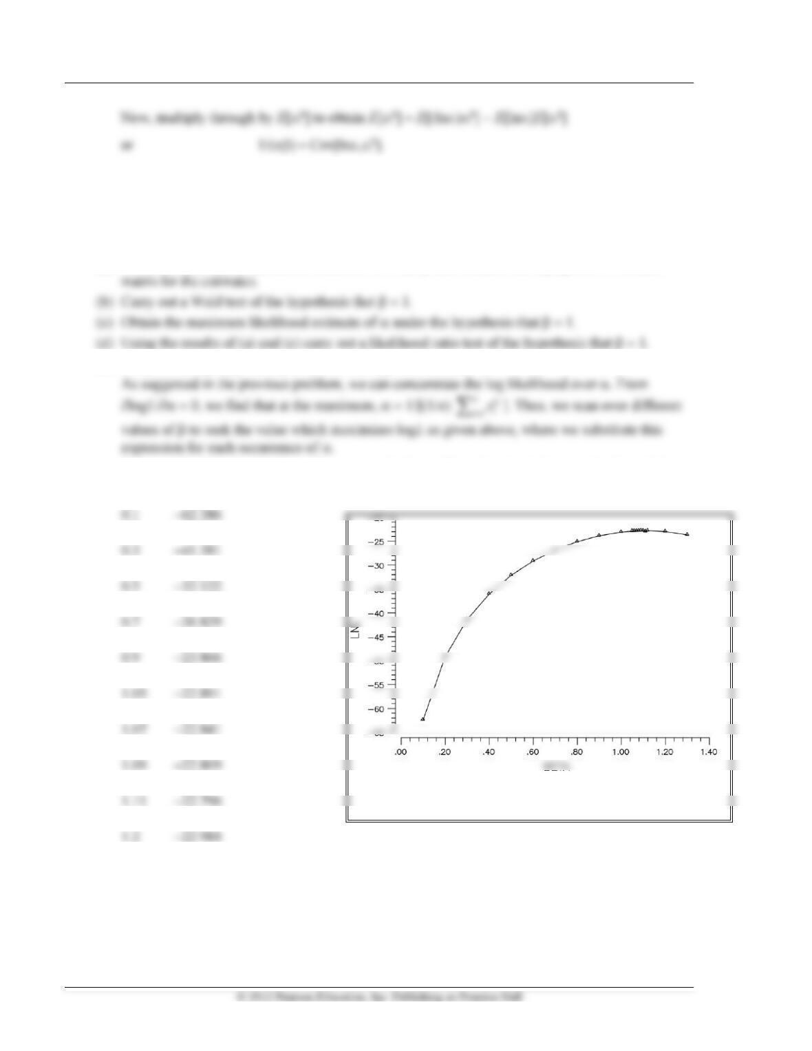
Values of and the log likelihood for a range of values of are listed and shown in the figure below.
logL
0.2 −49.175
0.4 −36.051
0.6 −29.127
0.8 −25.098
1.0 −23.101
1.06 −22.863
1.08 −22.823
1.10 −22.800
1.12 −22.797
1.3 −23.693
Appendix C Estimation and Inference 201
The maximum occurs at = 1.11. The implied value of is 1.179. The negative of
The Wald statistic for the hypothesis that = 1 is W = (1.11 − 1)2/0.041477 = 0.276. The critical
value for a test of size 0.05 is 3.84, so we would not reject the hypothesis.
Once again, this is a small value. To obtain the Lagrange multiplier statistic, we would compute
1
2 2 2
log /
log / log /
L
LL
−
− −
19. We consider forming a confidence interval for the variance of a normal distribution. As shown in
Example 4.29, the interval is formed by finding clower and cupper such that Prob[clower < 2[n−1] < cupper]
= 1 − .
The endpoints of the confidence interval are then (n − 1)s2/cupper and (n − 1)s2/clower. How do we find
the narrowest interval? Consider simply minimizing the width of the interval, cupper − clower subject to
20. Using the results in Example 4.26, and Section 4.7.2, estimate the asymptotic covariance matrix of
the method of moments estimators of P and based on
1
m−
and m2. (Note: You will need to use
the data in Table 4.1 to estimate V.)
Using the income data in Table 4.1, (1/n) times the covariance matrix of 1/xi and xi2 is