Appendix B
Probability and Distribution Theory
◼ Exercises
1. How many different 5-card poker hands can be dealt from a deck of 52 cards?
2. Compute the probability of being dealt 4 of a kind in a poker hand.
3. Suppose a lottery ticket costs $1 per play. The game is played by drawing six numbers without
replacement from the numbers 1 to 48. If you guess all six numbers, you win the prize. Now,
suppose that N = the number of tickets sold and P = the size of the prize. N and P are related by
N = 5 + 1.2P
P = 1 + 0.4N.
4. If x has a normal distribution with mean 1 and standard deviation 3, what are
(a) Prob[|x| > 2]?
(b) Prob[x > −1 | x < 1.5]?
Using the normal table,
(a) Prob[|x| > 2] = 1 − Prob[|x| 2]
176 Greene • Econometric Analysis, Seventh Edition
(b) Prob[x > −1 | x < 1.5] = Prob[−1 < x < 1.5]/Prob[x < 1.5]
5. Approximately what is the probability that a random variable with chi-squared distribution with 264
degrees of freedom is less than 297?
6. Chebychev inequality. For the following two probability distributions, find the lower limit of the
probability of the indicated event using the Chebychev inequality and the exact probability using the
appropriate table:
(a) x ~ Normal[0,32], and −4 < x < 4.
(b) x ~ chi-squared, 8 degrees of freedom, 0 < x < 16.
The inequality given in (3-18) states that Prob[|x − | < k ] > 1 − 1/k2. Note that the result is not
informative if k is less than or equal to 1.
7. Given the following joint probability distribution,
X
| 0 1 2
−−+−−−−−−−−−−−−−−−−−−
0| .05 .1 .03
Y 1| .21 .11 .19
2| .08 .15 .08
(a) Compute the following probabilities: Prob[Y < 2], Prob[Y < 2, X > 0], Prob[Y = 1, X > 1].
(b) Find the marginal distributions of X and Y.
(c) Calculate E[X], E[Y], Var[X], Var[Y], Cov[X,Y], and E[X2Y 3].
(d) Calculate Cov[Y,X2].
(e) What are the conditional distributions of Y given X = 2 and of X given Y > 0?
(f) Find E[Y|X] and Var[Y|X]. Obtain the two parts of the variance decomposition
Var[Y] = Ex[Var[Y|X]] + Varx[E[Y|X]].
We first obtain the marginal probabilities. For the joint distribution, these will be
X: P(0) = 0.34, P(1) = 0.36, P(2) = 0.30
Y: P(0) = 0.18, P(1) = 0.51, P(2) = 0.31.
Then,
Appendix B Probability and Distribution Theory 177
(c) E[X] = 0(0.34) + 1(0.36) + 2(0.30) = 0.96
(e) Prob[Y = 0 * X = 2] = 0.03/0.3 = 0.1
(f) E[Y * X = 0] = 0(0.05/0.34) + 1(0.21/0.34) + 2(0.08/0.34) = 1.088
8. Minimum mean squared error predictor. For the joint distribution in Exercise 7, compute E[y −
E[y|x]]2. Now, find the a and b which minimize the function E[y − a − bx]2. Given the solutions, verify

178 Greene • Econometric Analysis, Seventh Edition
Appendix B Probability and Distribution Theory 179
First, dividing by −2, then taking expectations produces
Solve the first for a = E[y] − bE[x] and substitute this in the second to obtain
The linear function compared to the conditional mean produces
Now, repeating the calculation above using a + bx instead of E[y|x] produces
(x = 0) (x = 1) (x = 2)
= 0.4950 > 0.4719.
9. Suppose x has an exponential distribution, f (x) = e−x, x > 0. Find the mean, variance, skewness, and
kurtosis of x. (The gamma integral will be useful for finding the raw moments.)
10. For the random variable in Exercise 9, what is the probability distribution of the random variable y = e−x?
What is E[y]? Prove that the distribution of this y is a special case of the beta distribution in (3-40).
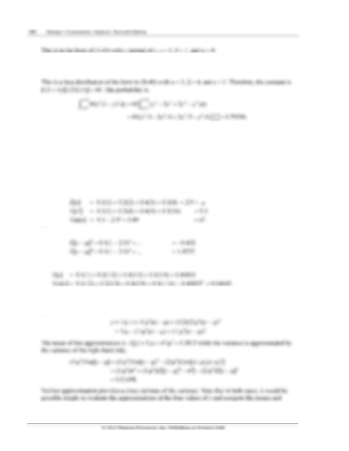
11. If the probability density of y is y2(1 − y)3 for y between 0 and 1, what is ? What is the probability
that y is between 0.25 and 0.75?
12. Suppose x has the following discrete probability distribution:
X 1 2 3 4
Prob[X = x] 0.1 0.2 0.4 0.3.
Find the exact mean and variance of X. Now, suppose Y = 1/X. Find the exact mean and variance of Y.
Find the mean and variance of the linear and quadratic approximations to Y = f (X). Are the mean and
variance of the quadratic approximation closer to the true mean than those of the linear approximation?
We will require a number of moments of x, which we derive first:
For later use, we also obtain
The approximation is y = 1/x. The exact mean and variance are
The linear Taylor series approximation around is y 1/ + (−1/2)(x − ). The mean of the linear
approximation is 1/ = 0.3448 while its variance is (1/4)Var[x−] = 2/4 = 0.01258. The quadratic
approximation is
Appendix B Probability and Distribution Theory 181
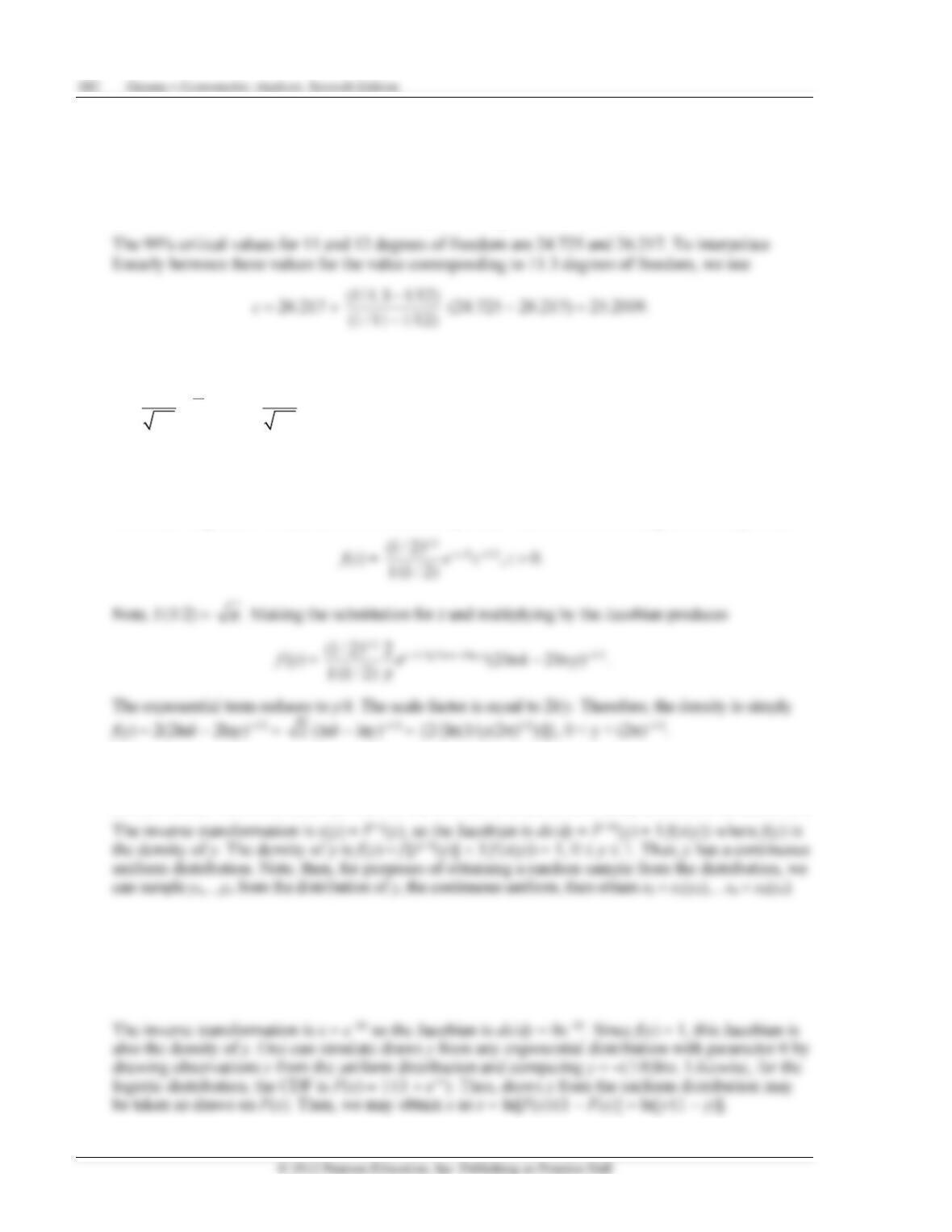
13. Interpolation in the chi–squared table. In order to find a percentage point in the chi-squared table which
is between two values, we interpolate linearly between the reciprocals of the degrees of freedom. The
chi–squared distribution is defined for noninteger values of the degrees of freedom parameter [see (3-39)],
but your table does not contain critical values for noninteger values. Using linear interpolation, find
the 99% critical value for a chi-squared variable with degrees of freedom parameter 11.3.
14. Suppose x has a standard normal distribution. What is the pdf of the following random variable?
2
2
11
,0 .
22
x
y e y
−
=
[Hints: You know the distribution of z = x2 from (C-30). The density of
this z is given in (C-39). Solve the problem in terms of y = g(z).]
We know that z = x2 is distributed as chi-squared with 1 degree of freedom. We seek the density of y = ke−z/2
where k = (2)−2. The inverse transformation is z = 2lnk − 2lny, so the Jacobian is |−2/y| = 2/y. The density
of z is that of gamma with parameters 1/2 and 1/2. [See (C-39) and the succeeding discussion.] Thus,
15. The fundamental probability transformation. Suppose that the continuous random variable x has
cumulative distribution F(x). What is the probability distribution of the random variable y = F(x)?
(Observation: This result forms the basis of the simulation of draws from many continuous distributions.)
16. Random number generators. Suppose x is distributed uniformly between 0 and 1, so f (x) = 1, 0 x 1.
Let be some positive constant. What is the pdf of y = −(1/)lnx? (Hint: See Section 3.5.) Does this
suggest a means of simulating draws from this distribution if one has a random number generator which
will produce draws from the uniform distribution? To continue, suggest a means of simulating draws
from a logistic distribution, f(x) = e−x/(1 + e−x)2.
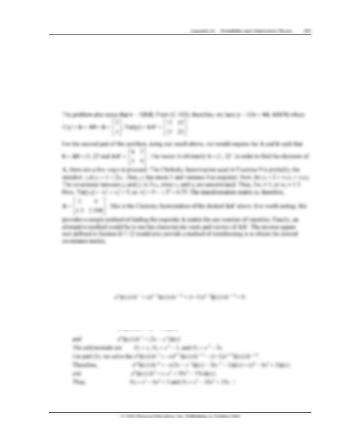
17. Suppose that x1 and x2 are distributed as independent standard normal. What is the joint distribution
of y1 = 2 + 3x1 + 2x2 and y2 = 4 + 5x1? Suppose you were able to obtain two samples of observations
from independent standard normal distributions. How would you obtain a sample from the bivariate
normal distribution with means 1 and 2 variances 4 and 9 and covariance 3?
We may write the pair of transformations as
y =
1
2
y
y
=
1
2
2 3 2
4 5 0
x
x
+
= b + Ax.
18. The density of the standard normal distribution, denoted (x), is given in (C-28). The function
based on the ith derivative of the density given by Hi = [(−1)idi (x)/dxi]/(x), i = 0,1,2,… is called a
Hermite polynomial. By definition, H0 = 1.
(a) Find the next three Hermite polynomials.
(b) A useful device in this context is the differential equation
Use this result and the results of part (a) to find H4 and H5.
The crucial result to be used in the derivations is d(x)/dx = −x(x). Therefore,
d 2(x)/dx 2 = (x 2 − 1)(x)
19. Continuation: orthogonal polynomials: The Hermite polynomials are orthogonal if x has a standard
normal distribution. That is, E[HiHj] = 0 if i j. Prove this for the H1, H2, and H3 which you obtained
above.
E[H1(x)H2(x)] = E[x(x2 − 1)] = E[x3 − x] = 0
20. If x and y have means x and y and variances
2
x
and
2
y
and covariance x y, what is the
approximation of the covariance matrix of the two random variables f1 = x/y and f2 = xy?
2
22
2
x
y xy x
x
+−
21. Factorial moments. For finding the moments of a distribution such as the Poisson, a useful device is
the factorial moment. (The Poisson distribution is given in Example 3.1.) The density is
f (x) = e−x/x!, x = 0,1,2,….
since the probabilities sum to 1. To find the variance, we will extend this method by finding E[x(x−1)],
and likewise for other moments. Use this method to find the variance and third central moment of
the Poisson distribution. (Note that this device is used to transform the factorial in the denominator
in the probability.)
Using the same technique,
E[x(x−1)] =
0( 1) ( )
xx x f x
=−
=
0( 1) / !
x
xx x e x
−
=−
Appendix B Probability and Distribution Theory 185
22. If x has a normal distribution with mean and standard deviation , what is the probability
distribution of y = e x?
23. If y has a log normal distribution, what is the probability distribution of y 2?
Let z = y2. Then, y =
z
and dy/dz
=
1/(2
z
). Inserting these in the density above, we find
24. Suppose y, x1, and x2 have a joint normal distribution with parameters x = [1, 2, 4] and covariance
matrix =
2 3 1
3 5 2 .
1 2 6
(a) Compute the intercept and slope in the function E[y*x1], Var[y*x1], and the coefficient of
(b) Compute the intercept and slopes in the conditional mean function, E[y*x1,x2]. What is
186 Greene • Econometric Analysis, Seventh Edition
We may just insert the figures above to obtain the results.
E[y*x1] = 1 + (3/5)(x1 − 2) = − 0.2 + 0.6x1,
25. What is the density of y = 1/x if x has a chi-squared distribution?
The density of a chi-squared variable is a gamma variable with parameters 1/2 and n/2 where n is the
degrees of freedom of the chi-squared variable. Thus,
26. What is the density and what are the mean and variance of y = 1/x if x has the gamma distribution
described in Section C.4.5?
The density of x is
1
( ) , 0.
P
xP
f x e x x
−−
=
If y = 1/x, then x = 1/y, and the Jacobian is |dx/dy| = 1/y2.
Appendix B Probability and Distribution Theory 187
27. Suppose x1 and x2 have the bivariate normal distribution described in Section 3.8. Consider an extension
of Example 3.4, where the bivariate normal distribution is obtained by transforming two independent
standard normal variables. Obtain the distribution of z = exp(y1)exp(y2) where y1 and y2 have a bivariate
28. Probability generating function. For a discrete random variable, x, the function
E[tx] =
Prob
0[]
x
xt X x
==
is called the probability generating function because in the function, the coefficient on ti is
Prob[X = i]. Suppose that x is the number of the repetitions of an experiment with probability
of success upon which the first success occurs. The density of x is the geometric distribution,
29. Moment generating function. For the random variable X, with probability density function f(x), if
the function M(t) = E[etx] exists, it is the moment generating function. Assuming the function exists,
it can be shown that drM(t)/dtr|t = 0 = E[xr ]. Find the moment generating functions for
(a) The exponential distribution of Exercise 9.
(b) The Poisson distribution of Exercise 21.
188 Greene • Econometric Analysis, Seventh Edition
For the Poisson distribution,
30. Moment generating function for a sum of variables. When it exists, the moment generating function
has a one to one correspondence with the distribution. Thus, for example, if we begin with some random
variable and find that a transformation of it has a particular MGF, we may infer that the function of
the random variable has the distribution associated with that MGF. A useful application is the following:
If x and y are independent, the MGF of x + y is Mx(t)My(t).
(a) Use this result to prove that the sum of Poisson random variables has a Poisson distribution.
(b) Use the result to prove that the sum of chi-squared variables has a chi-squared distribution.
[Note, you must first find the MGF for a chi-squared variate. The density is given in (3-39).]
(c) The MGF for the standard normal distribution is Mz = exp(−t2/2). Find the MGF for the N[,2]
distribution, then find the distribution of a sum of normally distributed variables.
(a) From the previous problem, Mx(t) = exp[(et − 1)]. Suppose y is distributed as Poisson
(b) The density of the chi–squared distribution with n degrees of freedom is [from (C-39)]
This is a gamma integral which reduces to M(t) = k(1/2 − t)−n/2(n/2). Now, reinserting the
constant k and simplifying produces the moment generating function M(t) = (1 − 2t)−n/2.
Appendix B Probability and Distribution Theory 189
(c) We let y = z + . Then, My(t) = E[exp(ty)] =
( ) ( )t z t tz t t z
E e e E e e E e
+
==