
7
Association Analysis:
Advanced Concepts
1. Consider the traffic accident data set shown in Table 7.1.
Table 7.1. Traffic accident data set.
Weather Driver’s Traffic Seat Belt Crash
Condition Condition Violation Severity
Good Alcohol-impaired Exceed speed limit No Major
Bad Sober None Yes Minor
Good Sober Disobey stop sign Yes Minor
Good Sober Exceed speed limit Yes Major
Bad Sober Disobey traffic signal No Major
Good Alcohol-impaired Disobey stop sign Yes Minor
Bad Alcohol-impaired None Yes Major
Good Sober Disobey traffic signal Yes Major
Good Alcohol-impaired None No Major
Bad Sober Disobey traffic signal No Major
Good Alcohol-impaired Exceed speed limit Yes Major
Bad Sober Disobey stop sign Yes Minor
(b) What is the maximum width of each transaction in the binarized data?
(c) Assuming that support threshold is 30%, how many candidate and fre-
quent itemsets will be generated?
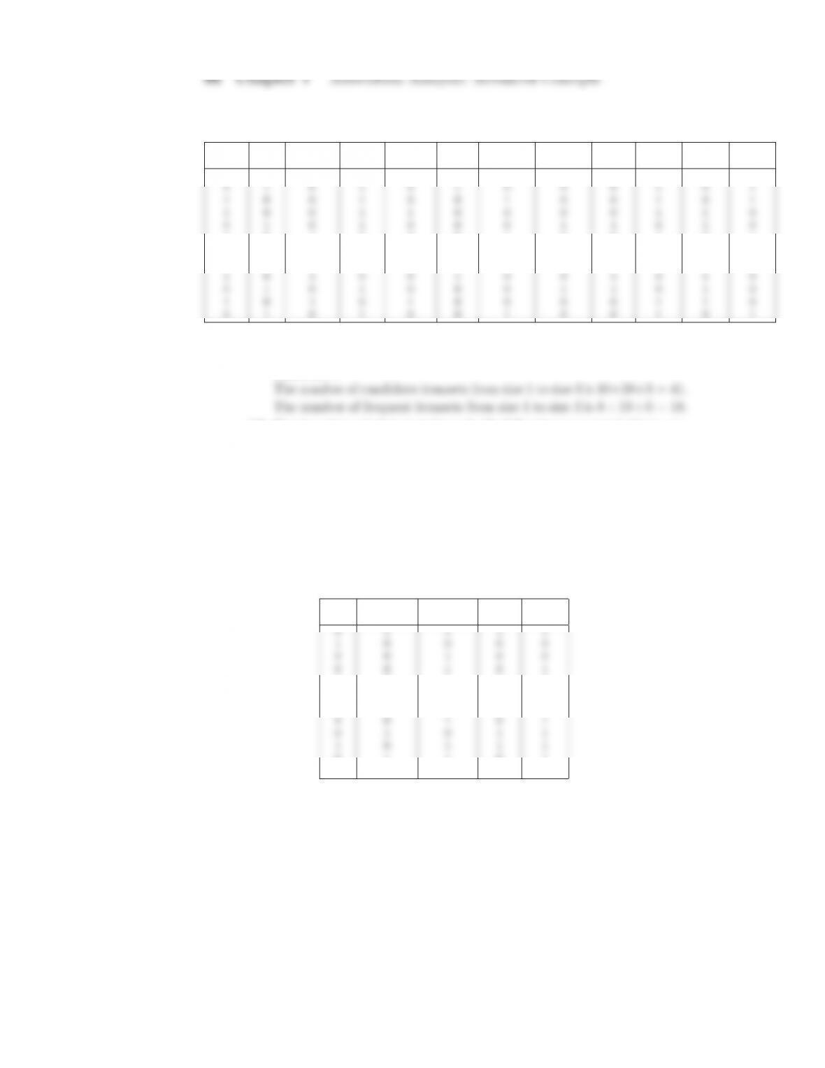
Table 7.2. Traffic accident data set.
Good Bad Alcohol Sober Exceed None Disobey Disobey Belt Belt Major Minor
speed stop traffic =No =Yes
1 0 1 0 1 0 0 0 1 0 1 0
1 0 1 0 0 0 1 0 0 1 0 1
0 1 1 0 0 1 0 0 0 1 1 0
1 0 0 1 0 0 0 1 0 1 1 0
Answer: 5
(d) Create a data set that contains only the following asymmetric binary at-
tributes: (Weather =Bad,Driver’s condition =Alcohol–impaired,
Traffic violation =Yes,Seat Belt =No,Crash Severity =Major).
For Traffic violation,onlyNone has a value of 0. The rest of the
attribute values are assigned to 1. Assuming that support threshold is
30%, how many candidate and frequent itemsets will be generated?
Answer:
The binarized data is shown in Table 7.3.
Table 7.3. Traffic accident data set.
Bad Alcohol Traffic Belt Major
Impaired violation =No
1 0 1 1 1
0 1 1 0 0
1 1 0 0 1
0 1 1 0 1
1 0 1 0 0
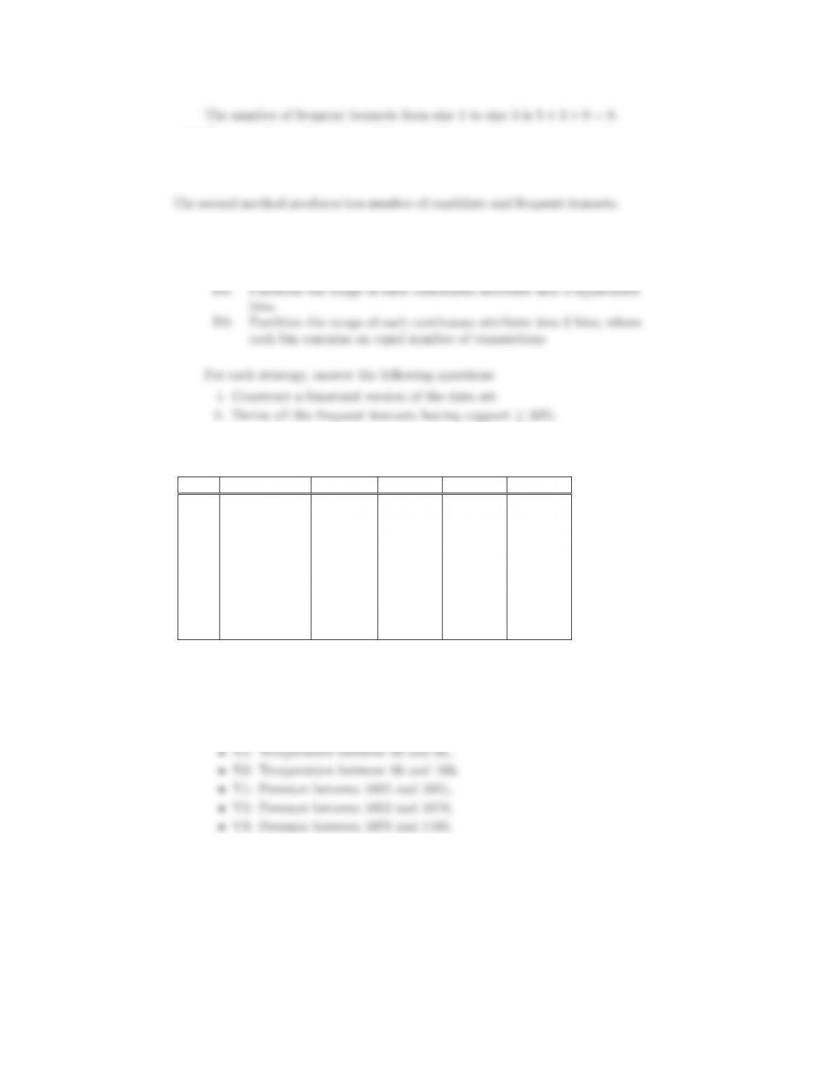
The number of candidate itemsets from size 1 to size 3 is 5+10+0 = 15.
97
(e) Compare the number of candidate and frequent itemsets generated in
parts (c) and (d).
Answer:
2. (a) Consider the data set shown in Table 7.4. Suppose we apply the fol-
lowing discretization strategies to the continuous attributes of the data
set.
Table 7.4. Data set for Exercise 2.
TID Temperature Pressure Alarm 1 Alarm 2 Alarm 3
195 1105 0 0 1
285 1040 1 1 0
3103 1090 1 1 1
497 1084 1 0 0
580 1038 0 1 1
6100 1080 1 1 0
783 1025 1 0 1
886 1030 1 0 0
9101 1100 1 1 1
Answer:
Table 7.5 shows the discretized data using D1, where the discretized
intervals are:
•X1: Temperature between 80 and 87,
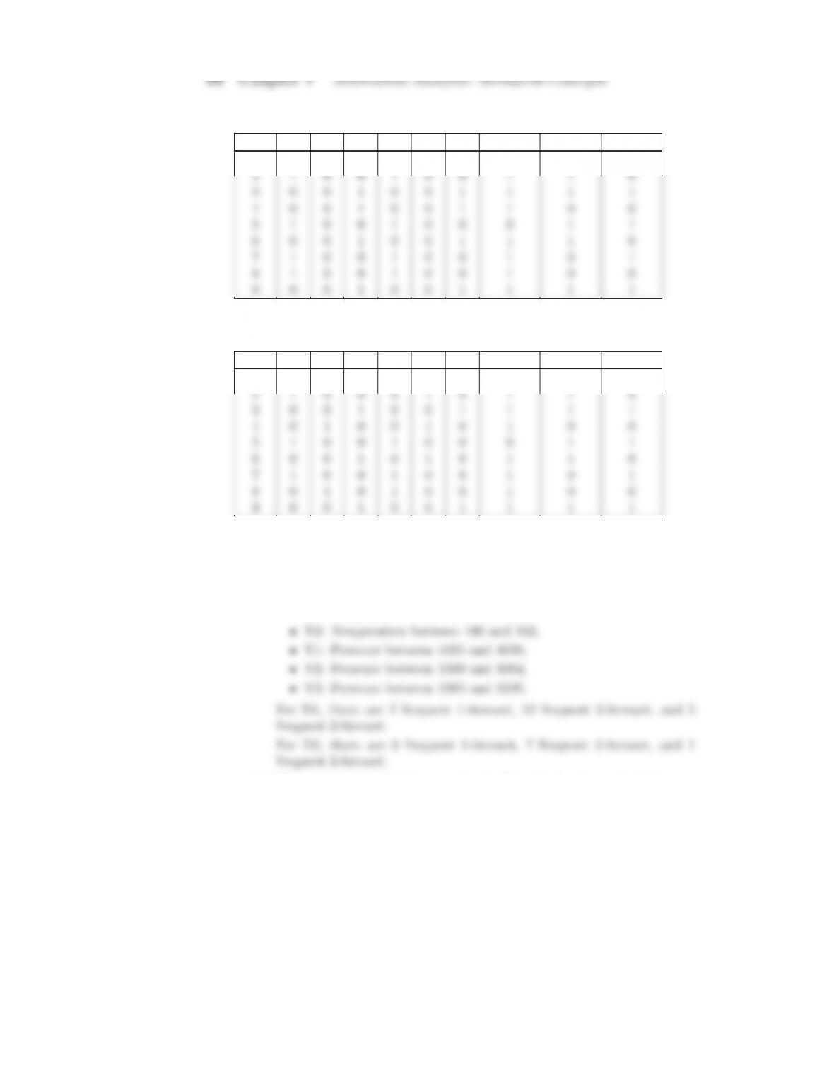
Table 7.5. Discretized data using D1.
TID X1 X2 X3 Y1 Y2 Y3 Alarm1 Alarm2 Alarm3
1 0 1 0 0 0 1 0 0 1
Table 7.6. Discretized data using D2.
TID X1 X2 X3 Y1 Y2 Y3 Alarm1 Alarm2 Alarm3
1 0 1 0 0 0 1 0 0 1
Table 7.6 shows the discretized data using D1, where the discretized
intervals are:
•X1: Temperature between 80 and 85,
•X2: Temperature between 86 and 97,
(b) The continuous attribute can also be discretized using a clustering ap-
proach.
i. Plot a graph of temperature versus pressure for the data points
shown in Table 7.4.
99
Answer:
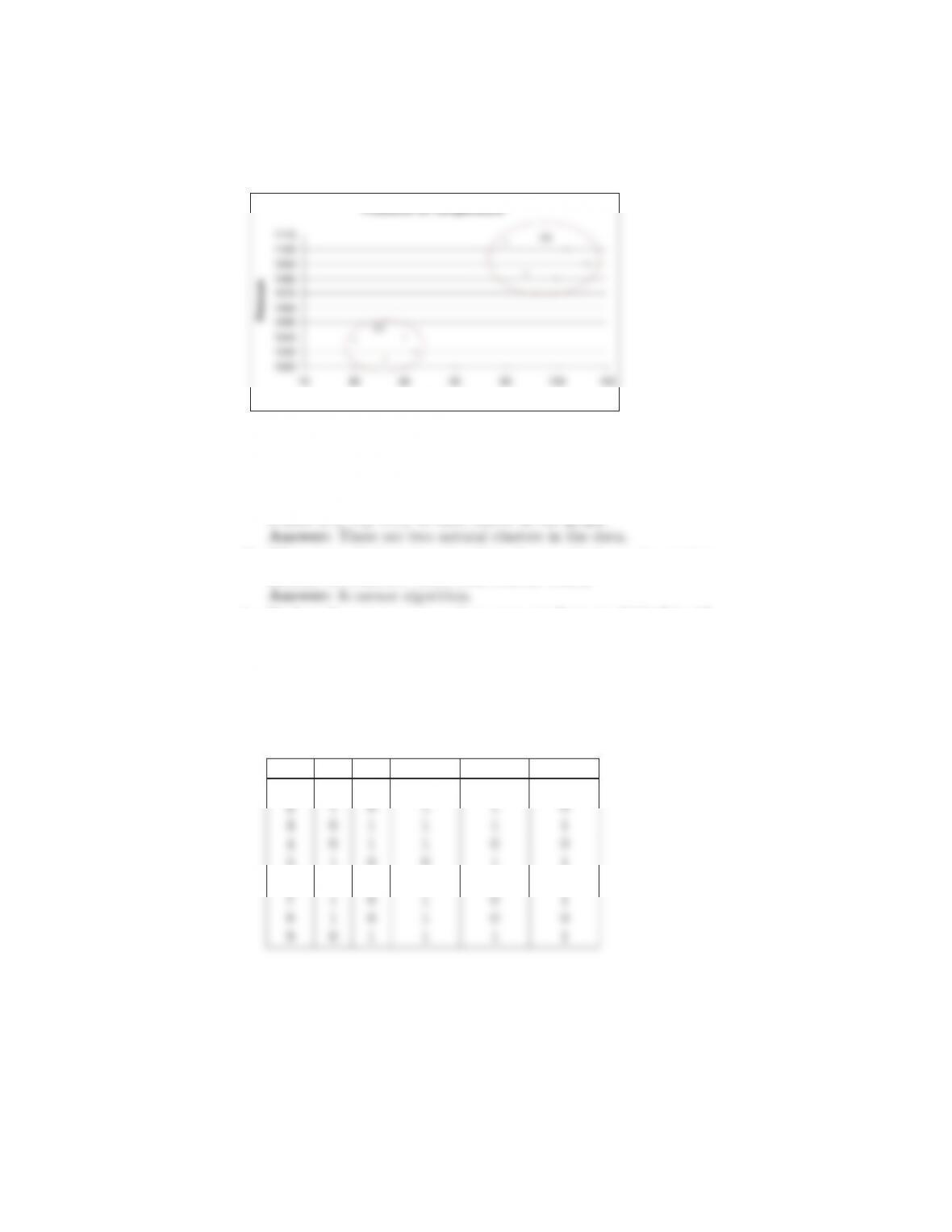
The graph of Temperature and Pressure is shown below.
Pressure vs Temperature
1030
1040
1050
1060
1070
1080
1090
1100
1110
Temperature
Pressure
C1
C2
Figure 7.1. Temperature versus Pressure.
ii. How many natural clusters do you observe from the graph? Assign
alabel(C1,C2, etc.) to each cluster in the graph.
iii. What type of clustering algorithm do you think can be used to
identify the clusters? State your reasons clearly.
iv. Replace the temperature and pressure attributes in Table 7.4 with
asymmetric binary attributes C1,C2, etc. Construct a transaction
matrix using the new attributes (along with attributes Alarm1,
Alarm2, and Alarm3).
Answer:
Table 7.7. Example of numeric data set.
TID C1 C2 Alarm1 Alarm2 Alarm3
1 0 1 0 0 1
5 1 0 0 1 1
6 0 1 1 1 0
100 Chapter 7 Association Analysis: Advanced Concepts
v. Derive all the frequent itemsets having support ≥30% from the
binarized data.
Answer:
3. Consider the data set shown in Table 7.8. The first attribute is continuous,
while the remaining two attributes are asymmetric binary. A rule is consid-
Table 7.8. Data set for Exercise 3.
A B C
1 1 1
2 1 1
3 1 0
4 1 0
5 1 1
6 0 1
7 0 0
8 1 1
9 0 0
10 0 0
11 0 0
12 0 1
(a) Compute the support and confidence for both rules.
Answer:
s({(1 ≤A≤2),B =1}→{C=1})=1/6
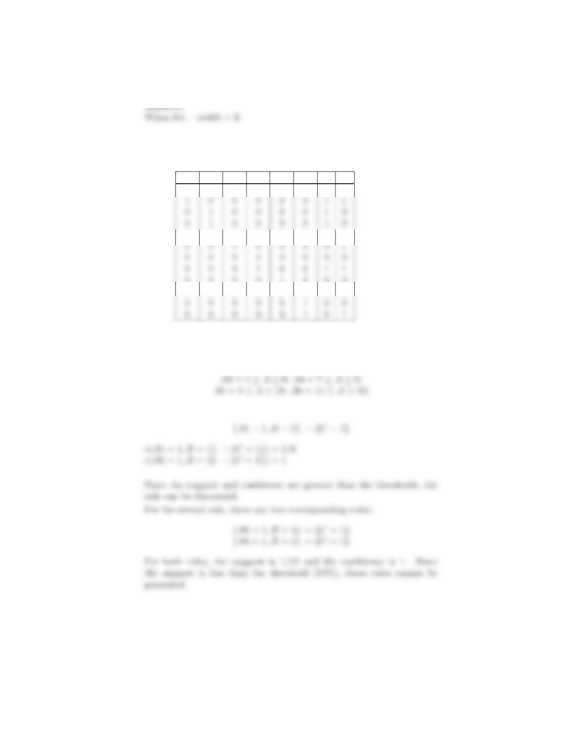
(b) To find the rules using the traditional Apriori algorithm, we need to
discretize the continuous attribute A. Suppose we apply the equal width
binning approach to discretize the data, with bin–width =2,3,4. For
each bin–width, state whether the above two rules are discovered by
the Apriori algorithm. (Note that the rules may not be in the same
exact form as before because it may contain wider or narrower intervals
101
for A.) For each rule that corresponds to one of the above two rules,
compute its support and confidence.
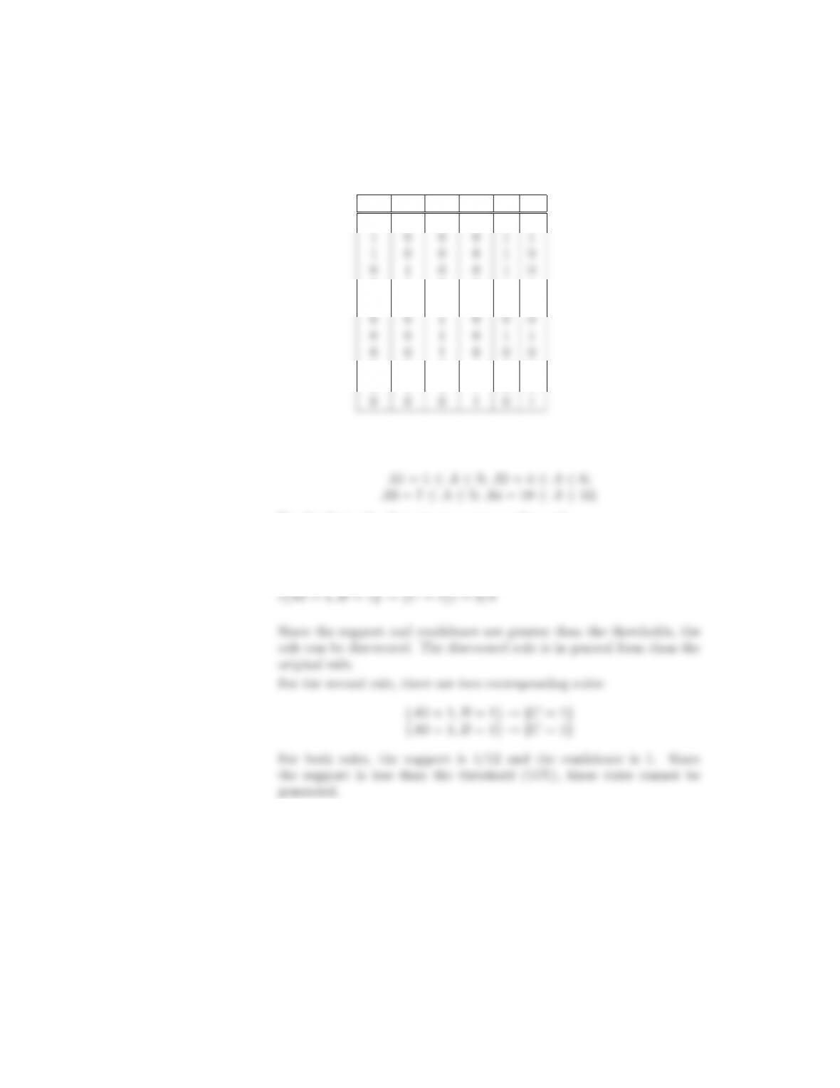
Table 7.9. A Synthetic Data set
A1 A2 A3 A4 A5 A6 B C
1 0 0 0 0 0 1 1
0 0 1 0 0 0 1 1
0 0 0 0 1 0 0 0
0 0 0 0 1 0 0 0
Where
A1=1≤A≤2; A2=3≤A≤4;
For the first rule, there is one corresponding rule:
102 Chapter 7 Association Analysis: Advanced Concepts
When bin −width =3:
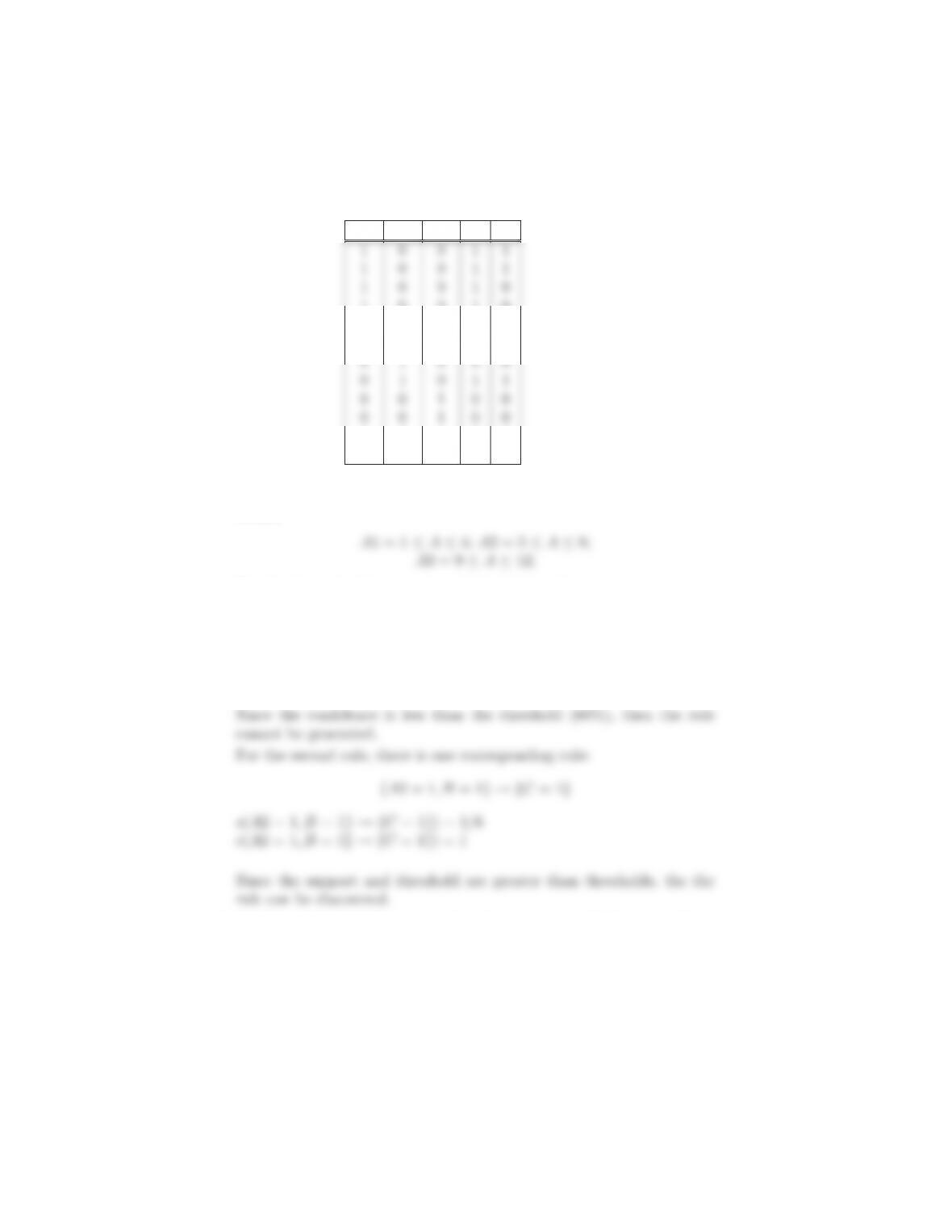
Table 7.10. A Synthetic Data set
A1 A2 A3 A4 B C
1 0 0 0 1 1
0 1 0 0 1 1
0 1 0 0 0 1
0 0 0 1 0 0
0 0 0 1 0 0
Where
For the first rule, there is one corresponding rule:
{A1=1,B =1}→{C=1}
s(A1=1,B =1}→{C=1})=1/6
103
When bin −width =4:
Table 7.11. A Synthetic Data set
A1 A2 A3 B C
1 0 0 1 0
0 1 0 1 1
0 1 0 0 1
0 0 1 0 0
0 0 1 0 1
Where
For the first rule, there is one correspomding rule:
{A1=1,B =1}→{C=1}
s(A1=1,B =1}→{C=1})=1/6
c(A1=1,B =1}→{C=1})=1/2
(c) Comment on the effectiveness of using the equal width approach for
classifying the above data set. Is there a bin-width that allows you to
104 Chapter 7 Association Analysis: Advanced Concepts
find both rules satisfactorily? If not, what alternative approach can you
take to ensure that you will find both rules?
Answer:
None of the discretization methods can effectively find both rules. One
approach to ensure that you can find both rules is to start with bin
4. Consider the data set shown in Table 7.12.
Table 7.12. Data set for Exercise 4.
Age Number of Hours Online per Week (B)
(A) 0–5 5–10 10 – 20 20 – 30 30 – 40
10 – 15 2 3 5 3 2
15 – 25 2 5 10 10 3
25 – 35 10 15 532
35 – 50 4 6 5 3 2
(a) For each combination of rules given below, specify the rule that has the
highest confidence.
i. 15 <A<25 −→ 10 <B<20, 10 <A<25 −→ 10 <B<20,
and 15 <A<35 −→ 10 <B<20.
Answer:
ii. 15 <A<25 −→ 10 <B<20, 15 <A<25 −→ 5<B<20, and
15 <A<25 −→ 5<B<30.
Answer:
iii. 15 <A<25 −→ 10 <B<20 and 10 <A<35 −→ 5<B<30.
Answer:
(b) Suppose we are interested in finding the average number of hours spent
online per week by Internet users between the age of 15 and 35. Write
the corresponding statistics-based association rule to characterize the
segment of users. To compute the average number of hours spent online,
105
approximate each interval by its midpoint value (e.g., use B=7.5to
represent the interval 5 <B<10).
Answer:
There are 65 people whose average age is between 15 and 35.
(c) Test whether the quantitative association rule given in part (b) is sta-
tistically significant by comparing its mean against the average number
of hours spent online by other users who do not belong to the age group.
For other users, the average number of hours spent online is:
5. For the data set with the attributes given below, describe how you would con-
vert it into a binary transaction data set appropriate for association analysis.
Specifically, indicate for each attribute in the original data set
(a) How many binary attributes it would correspond to in the transaction
data set,
(b) How the values of the original attribute would be mapped to values of
the binary attributes, and
(c) If there is any hierarchical structure in the data values of an attribute
that could be useful for grouping the data into fewer binary attributes.
The following is a list of attributes for the data set along with their possible
values. Assume that all attributes are collected on a per-student basis:
•Yea r : Freshman, Sophomore, Junior, Senior, Graduate:Masters, Grad-
uate:PhD, Professional
Answer:
106 Chapter 7 Association Analysis: Advanced Concepts
(a) Each attribute value can be represented using an asymmetric bi-
•Zip code : zip code for the home address of a U.S. student, zip code
for the local address of a non-U.S. student
Answer:
(a) Each attribute value is represented by an asymmetric binary at-
tribute. Therefore, we have as many asymmetric binary attributes
•College : Agriculture, Architecture, Continuing Education, Education,
Liberal Arts, Engineering, Natural Sciences, Business, Law, Medical,
Dentistry, Pharmacy, Nursing, Veterinary Medicine
Answer:
(a) Each attribute value is represented by an asymmetric binary at-
tribute. Therefore, we have as many asymmetric binary attributes
•On Campus : 1 if the student lives on campus, 0 otherwise
Answer:
•Each of the following is a separate attribute that has a value of 1 if the
person speaks the language and a value of 0, otherwise.
–Arabic
–Bengali
–Chinese Mandarin
–English
107
–Portuguese
–Russian
–Spanish
Answer:
(a) Each attribute value can be represented by an asymmetric bi-
nary attribute. Therefore, we have as many asymmetric binary
6. Consider the data set shown in Table 7.13. Suppose we are interested in
extracting the following association rule:
{α1≤Age ≤α2,Play Piano = Yes}−→{Enjoy Classical Music = Yes}
Table 7.13. Data set for Exercise 6.
Age Play Piano Enjoy Classical Music
9Yes Yes
17 Yes No
19 Yes Yes
21 No No
33 No No
To handle the continuous attribute, we apply the equal-frequency approach
with 3, 4, and 6 intervals. Categorical attributes are handled by introducing
as many new asymmetric binary attributes as the number of categorical val-
ues. Assume that the support threshold is 10% and the confidence threshold
is 70%.
(a) Suppose we discretize the Age attribute into 3 equal-frequency intervals.
Find a pair of values for α1and α2that satisfy the minimum support
and minimum confidence requirements.
108 Chapter 7 Association Analysis: Advanced Concepts
Answer:
(b) Repeat part (a) by discretizing the Age attribute into 4 equal-frequency
intervals. Compare the extracted rules against the ones you had ob-
tained in part (a).
Answer:
(c) Repeat part (a) by discretizing the Age attribute into 6 equal-frequency
intervals. Compare the extracted rules against the ones you had ob-
tained in part (a).
Answer:
(d) From the results in part (a), (b), and (c), discuss how the choice of
7. Consider the transactions shown in Table 7.14, with an item taxonomy given
in Figure 7.25.
Table 7.14. Example of market basket transactions.
Transaction ID Items Bought
1Chips, Cookies, Regular Soda, Ham
2Chips, Ham, Boneless Chicken, Diet Soda
3Ham, Bacon, Whole Chicken, Regular Soda
4Chips, Ham, Boneless Chicken, Diet Soda
5Chips, Bacon, Boneless Chicken
6Chips, Ham, Bacon, Whole Chicken, Regular Soda
7Chips, Cookies, Boneless Chicken, Diet Soda
(a) What are the main challenges of mining association rules with item
taxonomy?
Answer:
Difficulty of deciding the right support and confidence thresholds. Items

109
(b) Consider the approach where each transaction tis replaced by an ex-
tended transaction t′that contains all the items in tas well as their re-
spective ancestors. For example, the transaction t={Chips,Cookies}
will be replaced by t′={Chips,Cookies,Snack Food,Food}.Usethis
approach to derive all frequent itemsets (up to size 4) with support ≥
70%.
Answer:
There are 8 frequent 1-itemsets, 25 frequent 2-itemsets, 34 frequent
3-itemsets and 20 frequent 4-itemsets. The frequent 4-itemsets are:
{Food, Snack Food, Meat, Soda}{Food, Snack Food, Meat, Chips}
{Food, Snack Food, Meat, Pork}{Food, Snack Food, Meat, Chicken}
(c) Consider an alternative approach where the frequent itemsets are gen-
erated one level at a time. Initially, all the frequent itemsets involving
items at the highest level of the hierarchy are generated. Next, we use
the frequent itemsets discovered at the higher level of the hierarchy to
generate candidate itemsets involving items at the lower levels of the hi-
erarchy. For example, we generate the candidate itemset {Chips,Diet
Soda}only if {Snack Food,Soda}is frequent. Use this approach to
derive all frequent itemsets (up to size 4) with support ≥70%.
Answer:
There are 8 frequent 1-itemsets, 6 frequent 2-itemsets, and 1 frequent
3-itemset. The frequent 2-itemsets and 3-itemsets are:
(d) Compare the frequent itemsets found in parts (b) and (c). Comment
on the efficiency and completeness of the algorithms.
Answer:
8. The following questions examine how the support and confidence of an asso-
ciation rule may vary in the presence of a concept hierarchy.