
5
Classification:
Alternative Techniques
1. Consider a binary classification problem with the following set of attributes
and attribute values:
•Air Conditioner = {Working, Broken}
•Engine = {Good, Bad}
•Mileage = {High, Medium, Low}
•Rust = {Yes, No}
Suppose a rule-based classifier produces the following rule set:
Mileage = High −→ Value = Low
Mileage = Low −→ Value = High
Air Conditioner = Working, Engine = Good −→ Value = High
Air Conditioner = Working, Engine = Bad −→ Value = Low
Air Conditioner = Broken −→ Value = Low
(a) Are the rules mutually exclustive?
(b) Is the rule set exhaustive?
(c) Is ordering needed for this set of rules?
(d) Do you need a default class for the rule set?

2. The RIPPER algorithm (by Cohen [1]) is an extension of an earlier algorithm
called IREP (by F¨urnkranz and Widmer [3]). Both algorithms apply the
reduced-error pruning method to determine whether a rule needs to be
pruned. The reduced error pruning method uses a validation set to estimate
the generalization error of a classifier. Consider the following pair of rules:
R1:A−→ C
R2:A∧B−→ C
R2is obtained by adding a new conjunct, B, to the left-hand side of R1.For
this question, you will be asked to determine whether R2is preferred over
R1from the perspectives of rule-growing and rule-pruning. To determine
whether a rule should be pruned, IREP computes the following measure:
vIREP =p+(N−n)
P+N,
where Pis the total number of positive examples in the validation set, Nis
the total number of negative examples in the validation set, pis the number
of positive examples in the validation set covered by the rule, and nis the
number of negative examples in the validation set covered by the rule. vIREP
is actually similar to classification accuracy for the validation set. IREP
favors rules that have higher values of vIREP . On the other hand, RIPPER
applies the following measure to determine whether a rule should be pruned:
vRIPPER =p−n
p+n.
(a) Suppose R1is covered by 350 positive examples and 150 negative ex-
amples, while R2is covered by 300 positive examples and 50 negative
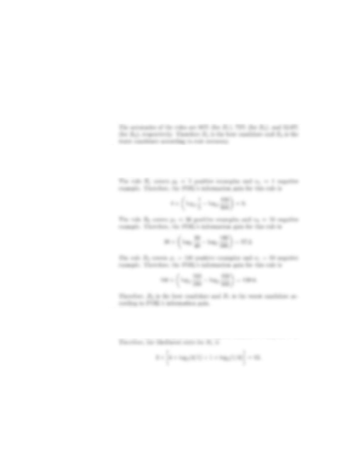
examples. Compute the FOIL’s information gain for the rule R2with
respect to R1.
Answer:
For this problem, p0= 350, n0= 150, p1= 300, and n1= 50. There-
(b) Consider a validation set that contains 500 positive examples and 500
negative examples. For R1, suppose the number of positive examples
covered by the rule is 200, and the number of negative examples covered
by the rule is 50. For R2, suppose the number of positive examples
covered by the rule is 100 and the number of negative examples is 5.
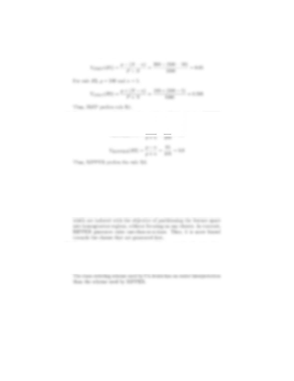
Compute vIREP for both rules. Which rule does IREP prefer?
47
Answer:
For this problem, P= 500, and N= 500.
For rule R1, p= 200 and n= 50. Therefore,
(c) Compute vRIPPER for the previous problem. Which rule does RIPPER
prefer?
Answer:
VRIPPER(R1) = p−n
3. C4.5rules is an implementation of an indirect method for generating rules
from a decision tree. RIPPER is an implementation of a direct method for
generating rules directly from data.
(a) Discuss the strengths and weaknesses of both methods.
Answer:
The C4.5 rules algorithm generates classification rules from a global
perspective. This is because the rules are derived from decision trees,
(b) Consider a data set that has a large difference in the class size (i.e.,
some classes are much bigger than others). Which method (between
C4.5rules and RIPPER) is better in terms of finding high accuracy
rules for the small classes?
Answer:
48 Chapter 5 Classification: Alternative Techniques
4. Consider a training set that contains 100 positive examples and 400 negative
examples. For each of the following candidate rules,
R1:A−→ + (covers 4 positive and 1 negative examples),
R2:B−→ + (covers 30 positive and 10 negative examples),
R3:C−→ + (covers 100 positive and 90 negative examples),
determine which is the best and worst candidate rule according to:
(a) Rule accuracy.
Answer:
(b) FOIL’s information gain.
Answer:
Assume the initial rule is ∅−→+. This rule covers p0= 100 positive
examples and n0= 400 negative examples.
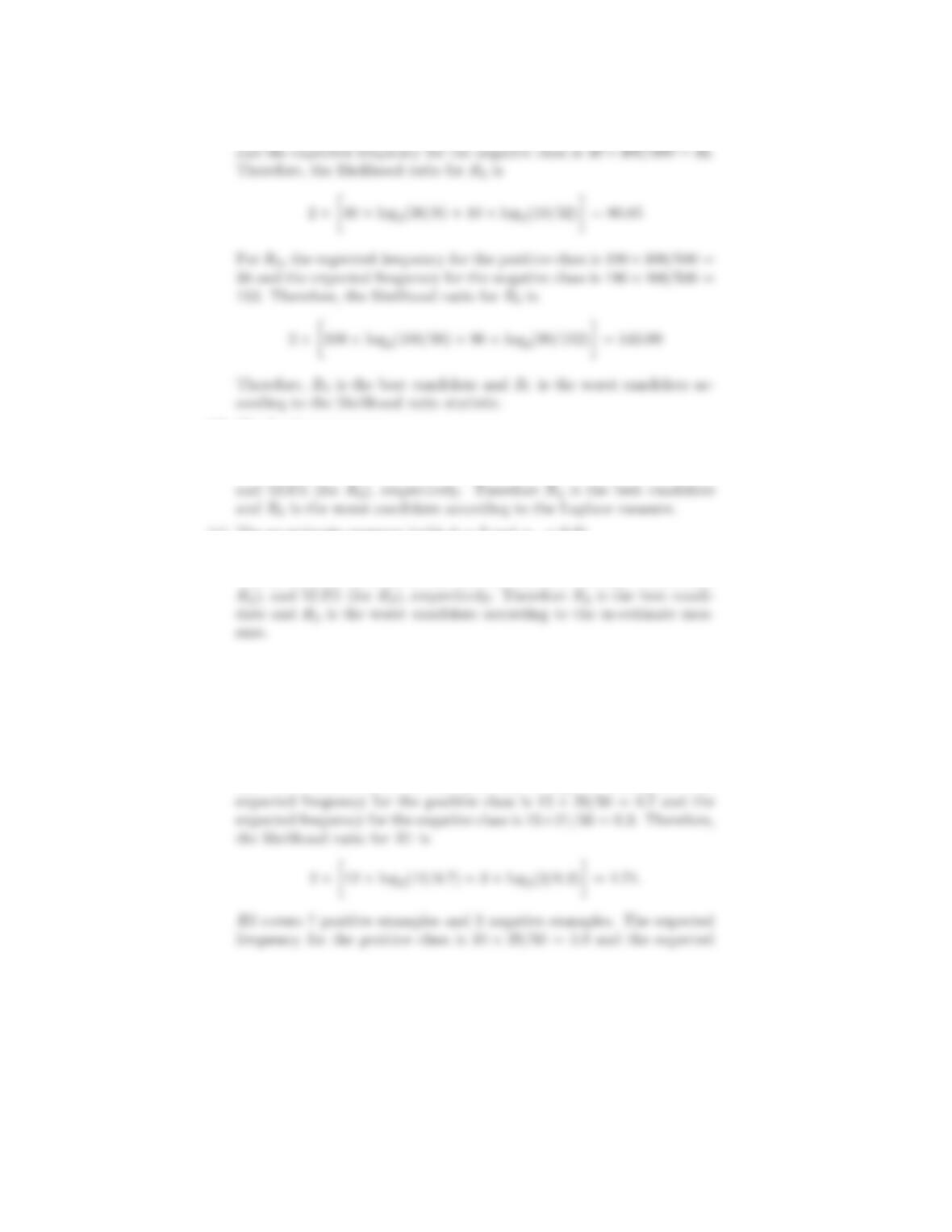
(c) The likelihood ratio statistic.
Answer:
For R1, the expected frequency for the positive class is 5 ×100/500 = 1
and the expected frequency for the negative class is 5 ×400/500 = 4.
49
For R2, the expected frequency for the positive class is 40×100/500 = 8
(d) The Laplace measure.
Answer:
The Laplace measure of the rules are 71.43% (for R1), 73.81% (for R2),
(e) The m-estimate measure (with k=2andp+=0.2).
Answer:
The m-estimate measure of the rules are 62.86% (for R1), 73.38% (for
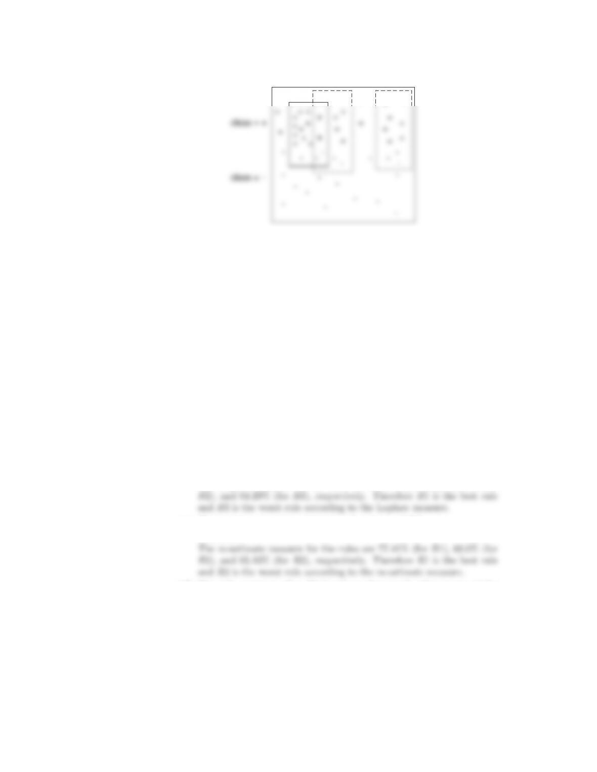
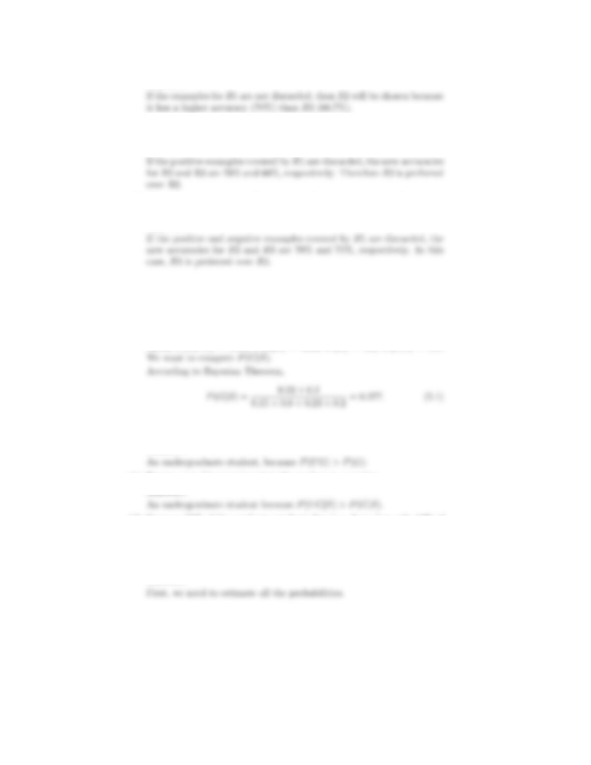
5. Figure 5.1 illustrates the coverage of the classification rules R1, R2, and R3.
Determine which is the best and worst rule according to:
(a) The likelihood ratio statistic.
Answer:
There are 29 positive examples and 21 negative examples in the data
set. R1 covers 12 positive examples and 3 negative examples. The
50 Chapter 5 Classification: Alternative Techniques
++ + ++
R1
R3 R2
Figure 5.1. Elimination of training records by the sequential covering algorithm.
R1
,
R2
, and
R3
represent regions covered by three different rules.
frequency for the negative class is 10 ×21/50 = 4.2. Therefore, the
likelihood ratio for R2is
2×7×log2(7/5.8) + 3 ×log2(3/4.2)=0.89.
R3 covers 8 positive examples and 4 negative examples. The expected
frequency for the positive class is 12 ×29/50 = 6.96 and the expected
frequency for the negative class is 12 ×21/50 = 5.04. Therefore, the
likelihood ratio for R3is
2×8×log2(8/6.96) + 4 ×log2(4/5.04)=0.5472.
R1 is the best rule and R3 is the worst rule according to the likelihood
ratio statistic.
(b) The Laplace measure.
Answer:
The Laplace measure for the rules are 76.47% (for R1), 66.67% (for
(c) The m-estimate measure (with k=2andp+=0.58).
Answer:
(d) The rule accuracy after R1 has been discovered, where none of the
examples covered by R1 are discarded).
51
Answer:
(e) The rule accuracy after R1 has been discovered, where only the positive
examples covered by R1 are discarded).
Answer:
(f) The rule accuracy after R1 has been discovered, where both positive
and negative examples covered by R1 are discarded.
Answer:
6. (a) Suppose the fraction of undergraduate students who smoke is 15% and
the fraction of graduate students who smoke is 23%. If one-fifth of the
college students are graduate students and the rest are undergraduates,
what is the probability that a student who smokes is a graduate student?
Answer:
Given P(S|UG)=0.15, P(S|G)=0.23, P(G)=0.2, P(UG)=0.8.
(b) Given the information in part (a), is a randomly chosen college student
more likely to be a graduate or undergraduate student?
Answer:
(c) Repeat part (b) assuming that the student is a smoker.
Answer:
(d) Suppose 30% of the graduate students live in a dorm but only 10% of
the undergraduate students live in a dorm. If a student smokes and lives
in the dorm, is he or she more likely to be a graduate or undergraduate
student? You can assume independence between students who live in
a dorm and those who smoke.
Answer:

52 Chapter 5 Classification: Alternative Techniques
P(D|UG)=0.1, P(D|G)=0.3.
P(D)=P(UG).P (D|UG)+P(G).P (D|G)=0.8∗0.1+0.2∗0.3=0.14.
P(S)=P(S|UG)P(UG)+P(S|G)P(G)=0.15∗0.8+0.23∗0.2=0.166.
P(DS|G)=P(D|G)×P(S|G)=0.3×0.23 = 0.069 (using conditional
independent assumption)
P(DS|UG)=P(D|UG)×P(S|UG)=0.1×0.15 = 0.015.
We need to compute P(G|DS)andP(UG|DS).
P(G|DS)=0.069 ×0.2
P(DS)=0.0138
P(DS)
P(UG|DS)=0.015 ×0.8
P(DS)=0.012
P(DS)
Since P(G|DS)>P(UG|DS), he/she is more likely to be a graduate
student.
7. Consider the data set shown in Table 5.1
Table 5.1. Data set for Exercise 7.
Record A B C Class
1 0 0 0 +
2 0 0 1 −
3 0 1 1 −
4 0 1 1 −
5 0 0 1 +
6 1 0 1 +
7 1 0 1 −
8 1 0 1 −
9 1 1 1 +
10 1 0 1 +
(a) Estimate the conditional probabilities for P(A|+), P(B|+), P(C|+),
P(A|−), P(B|−), and P(C|−).
Answer:
P(A=1|−)=2/5=0.4, P(B=1|−)=2/5=0.4,
53
(b) Use the estimate of conditional probabilities given in the previous ques-
tion to predict the class label for a test sample (A=0,B =1,C =0)
using the na¨ıve Bayes approach.
Answer:
Let P(A=0,B =1,C =0)=K.
P(+|A=0,B =1,C =0)
=P(A=0,B =1,C =0|+) ×P(+)
P(A=0,B =1,C =0)
(c) Estimate the conditional probabilities using the m-estimate approach,
with p=1/2andm=4.
Answer:
P(A=0|+) = (2 + 2)/(5 + 4) = 4/9,
P(A=0|−)=(3+2)/(5 + 4) = 5/9,
(d) Repeat part (b) using the conditional probabilities given in part (c).
54 Chapter 5 Classification: Alternative Techniques
P(+|A=0,B =1,C =0)
=P(A=0,B =1,C =0|+) ×P(+)
(e) Compare the two methods for estimating probabilities. Which method
is better and why?
Answer:
8. Consider the data set shown in Table 5.2.
(a) Estimate the conditional probabilities for P(A=1|+), P(B=1|+),
P(C=1|+), P(A=1|−), P(B=1|−), and P(C=1|−) using the
same approach as in the previous problem.
Answer:
(b) Use the conditional probabilities in part (a) to predict the class label for
a test sample (A=1,B =1,C =1)usingthena¨ıve Bayes approach.
Answer:
Table 5.2. Data set for Exercise 8.
Instance A B C Class
1 0 0 1 −
2 1 0 1 +
3 0 1 0 −
4 1 0 0 −
5 1 0 1 +
6 0 0 1 +
7 1 1 0 −
8 0 0 0 −
9 0 1 0 +
10 1 1 1 +
P(+|R)=P(R|+)P(+)/P (R)andP(−|R)=P(R|−)P(−)/P (R).
Since P(+) = P(−)=0.5andP(R) is constant, Rcan be classified by
comparing P(+|R)andP(−|R).
For this question,
P(R|+) = P(A=1|+) ×P(B=1|+) ×P(C=1|+) = 0.192
P(R|−)=P(A=1|−)×P(B=1|−)×P(C=1|−)=0.032
Since P(R|+) is larger, the record is assigned to (+) class.
(c) Compare P(A=1),P(B=1),andP(A=1,B = 1). State the
relationships between Aand B.
Answer:
(d) Repeat the analysis in part (c) using P(A=1),P(B=0),andP(A=
1,B =0).
Answer:
(e) Compare P(A=1,B =1|Class = +) against P(A=1|Class =+)
and P(B=1|Class = +). Are the variables conditionally independent
given the class?
Answer:
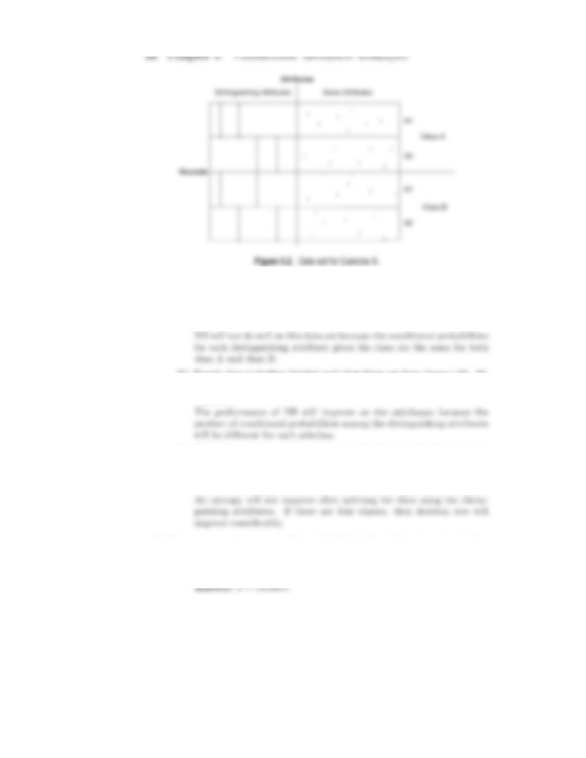
9. (a) Explain how na¨ıve Bayes performs on the data set shown in Figure 5.2.
Answer:
(b) If each class is further divided such that there are four classes (A1, A2,
B1, and B2), will na¨ıve Bayes perform better?
Answer:
(c) How will a decision tree perform on this data set (for the two-class
problem)? What if there are four classes?
Answer:
For the two-class problem, decision tree will not perform well because
10. Repeat the analysis shown in Example 5.3 for finding the location of a decision
boundary using the following information:
(a) The prior probabilities are P(Crocodile)=2×P(Alligator).
57
(b) The prior probabilities are P(Alligator)=2×P(Crocodile).
(c) The prior probabilities are the same, but their standard deviations are
different; i.e., σ(Crocodile)=4andσ(Alligator)=2.
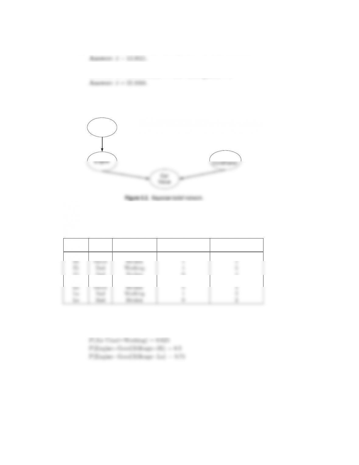
11. Figure 5.3 illustrates the Bayesian belief network for the data set shown in
Table 5.3. (Assume that all the attributes are binary).
Mileage
Air
Table 5.3. Data set for Exercise 11.
Mileage Engine Air Conditioner Number of Records Number of Records
with Car Value=Hi with Car Value=Lo
Hi Good Working 3 4
Hi Bad Broken 0 4
Lo Good Working 9 0
(a) Draw the probability table for each node in the network.
P(Mileage=Hi) = 0.5