58 Chapter 5 Classification: Alternative Techniques
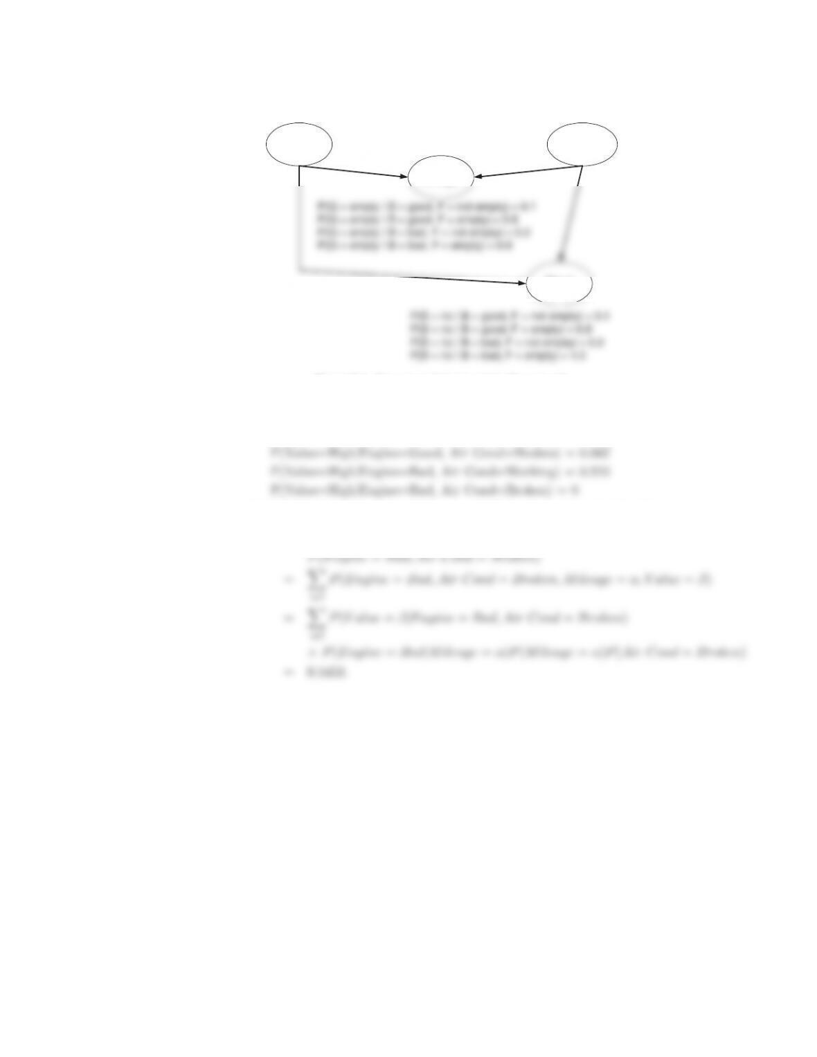
Battery
Gauge
Fuel
P(B = bad) = 0.1 P(F = empty) = 0.2
Figure 5.4. Bayesian belief network for Exercise 12.
P(Value=High|Engine=Good, Air Cond=Working) = 0.750
(b) Use the Bayesian network to compute P(Engine = Bad, Air Conditioner
=Broken).
12. Given the Bayesian network shown in Figure 5.4, compute the following prob-
abilities:
(a) P(B=good,F=empty,G=empty,S=yes).

59
Answer:
P(B=good, F =empty, G =empty, S =yes)
(b) P(B=bad,F=empty,G=notempty,S=no).
Answer:
(c) Given that the battery is bad, compute the probability that the car will
start.
Answer:
P(S=yes|B=bad)
13. Consider the one-dimensional data set shown in Table 5.4.
Table 5.4. Data set for Exercise 13.
x0.5 3.0 4.5 4.6 4.9 5.2 5.3 5.5 7.0 9.5
y−−+++− − +− −
(a) Classify the data point x=5.0 according to its 1-, 3-, 5-, and 9-nearest
neighbors (using majority vote).
Answer:
1-nearest neighbor: +,
(b) Repeat the previous analysis using the distance-weighted voting ap-
proach described in Section 5.2.1.

60 Chapter 5 Classification: Alternative Techniques
Answer:
1-nearest neighbor: +,
14. The nearest-neighbor algorithm described in Section 5.2 can be extended to
handle nominal attributes. A variant of the algorithm called PEBLS (Parallel
Examplar-Based Learning System) by Cost and Salzberg [2] measures the
distance between two values of a nominal attribute using the modified value
difference metric (MVDM). Given a pair of nominal attribute values, V1and
V2, the distance between them is defined as follows:
d(V1,V
2)=
k
i=1
ni1
n1−ni2
n2
,(5.2)
where nij is the number of examples from class iwith attribute value Vjand
njis the number of examples with attribute value Vj.
Consider the training set for the loan classification problem shown in Figure
5.9. Use the MVDM measure to compute the distance between every pair of
attribute values for the Home Owner and Marital Status attributes.
Answer:
The training set shown in Figure 5.9 can be summarized for the Home Owner
and Marital Status attributes as follows.
15. For each of the Boolean functions given below, state whether the problem is
linearly separable.
(a) AAND BAND C
(b) NOT AAND B
(c) (AOR B) AND (AOR C)
(d) (AXOR B) AND (AOR B)
16. (a) Demonstrate how the perceptron model can be used to represent the
AND and OR functions between a pair of Boolean variables.
Answer:
Let x1and x2be a pair of Boolean variables and ybe the output. For
AND function, a possible perceptron model is:
(b) Comment on the disadvantage of using linear functions as activation
functions for multilayer neural networks.
Answer:
Multilayer neural networks is useful for modeling nonlinear relation-
17. You are asked to evaluate the performance of two classification models, M1
and M2. The test set you have chosen contains 26 binary attributes, labeled
as Athrough Z.
Table 5.5 shows the posterior probabilities obtained by applying the models to
the test set. (Only the posterior probabilities for the positive class are shown).
As this is a two-class problem, P(−)=1−P(+) and P(−|A,…,Z)=1−
P(+|A,…,Z). Assume that we are mostly interested in detecting instances
from the positive class.
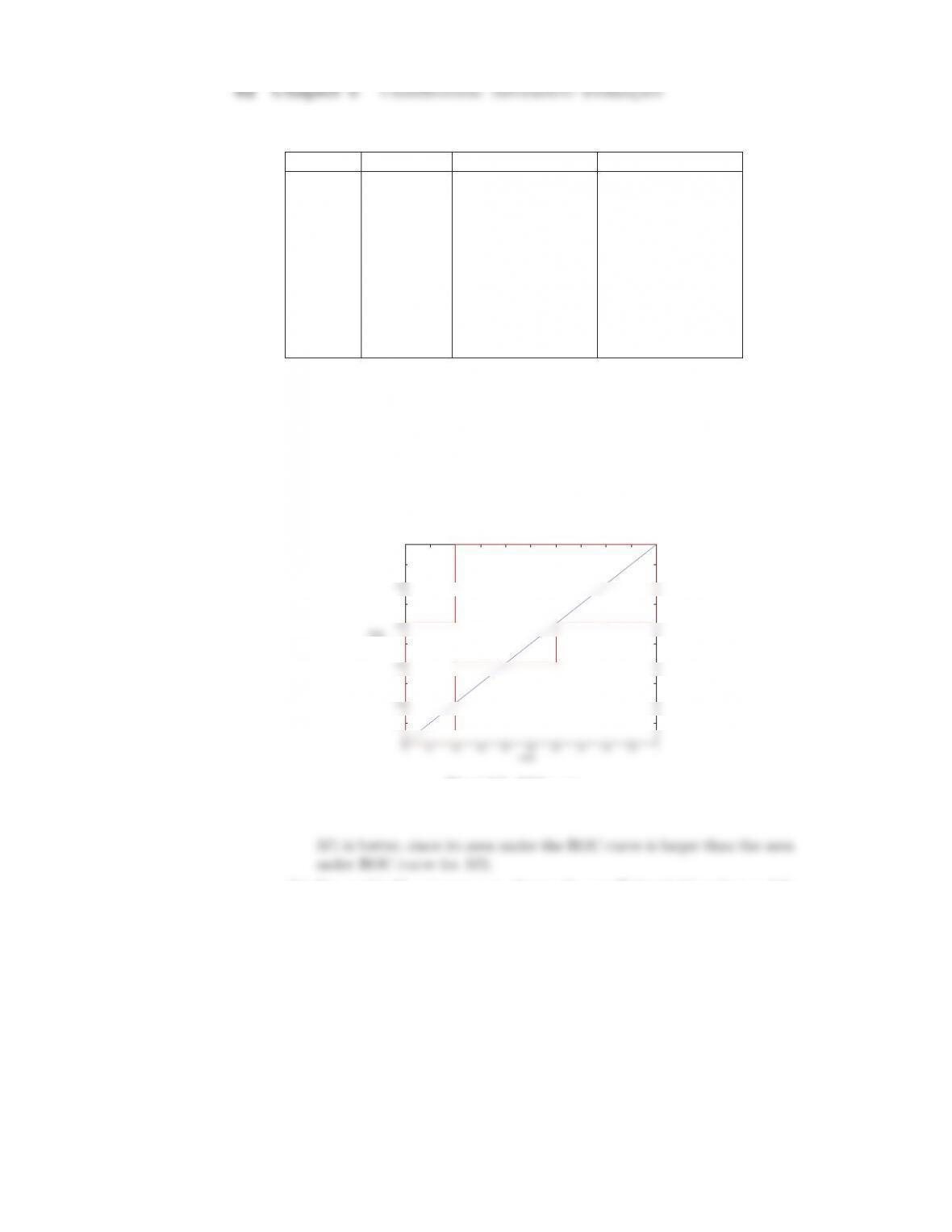
Table 5.5. Posterior probabilities for Exercise 17.
Instance True Class P(+|A,…,Z,M
1)P(+|A,…,Z,M
2)
1 + 0.73 0.61
2 + 0.69 0.03
3−0.44 0.68
4−0.55 0.31
5 + 0.67 0.45
6 + 0.47 0.09
7−0.08 0.38
8−0.15 0.05
9 + 0.45 0.01
10 −0.35 0.04
(a) Plot the ROC curve for both M1and M2. (You should plot them on
the same graph.) Which model do you think is better? Explain your
reasons.
Answer:
TheROCcurveforM1andM2 are shown in the Figure 5.5.
0 0.1 0.2 0.3 0.4 0.5 0.6 0.7 0.8 0.9 1
0
0.1
0.3
0.5
0.7
0.9
1
M1 M2
TPR
Figure 5.5. ROC curve.
(b) For model M1, suppose you choose the cutoff threshold to be t=0.5.
In other words, any test instances whose posterior probability is greater
than twill be classified as a positive example. Compute the precision,
recall, and F-measure for the model at this threshold value.

63
When t=0.5, the confusion matrix for M1 is shown below.
(c) Repeat the analysis for part (c) using the same cutoff threshold on
model M2.ComparetheF-measure results for both models. Which
model is better? Are the results consistent with what you expect from
the ROC curve?
Answer:
When t=0.5, the confusion matrix for M2 is shown below.
+ –
Actual + 1 4
(d) Repeat part (c) for model M1using the threshold t=0.1. Which
threshold do you prefer, t=0.5ort=0.1? Are the results consistent
with what you expect from the ROC curve?
Answer:
When t=0.1, the confusion matrix for M1 is shown below.
+ –
t=0.5, FPR =0.2andTRP =0.6. Since (0.2, 0.6) is closer to the
point (0, 1), we favor t=0.5. This result is inconsistent with the results

64 Chapter 5 Classification: Alternative Techniques
18. Following is a data set that contains two attributes, Xand Y,andtwoclass
labels, “+” and “−”. Each attribute can take three different values: 0,1, or
2.
X Y
Number of
Instances
+−
0 0 0 100
1 0 0 0
2 0 0 100
0 1 10 100
1 1 10 0
2 1 10 100
0 2 0 100
1 2 0 0
2 2 0 100
The concept for the “+” class is Y= 1 and the concept for the “−”classis
X=0∨X=2.
(a) Build a decision tree on the data set. Does the tree capture the “+”
and “−” concepts?
Answer:
There are 30 positive and 600 negative examples in the data. Therefore,
at the root node, the error rate is
65
Y=0 Y=1 Y=2
EY=0 =0
(b) What are the accuracy, precision, recall, and F1-measure of the decision
tree? (Note that precision, recall, and F1-measure are defined with
respect to the “+” class.)
Answer: The confusion matrix on the training data:
accuracy : 610
630 =0.9683
(c) Build a new decision tree with the following cost function:
C(i, j)=⎧
⎨
⎩
0,if i=j;
1,if i=+,j=−;
Number of −instances
Number of + instances ,if i=−,j=+.
(Hint: only the leaves of the old decision tree need to be changed.)
Does the decision tree capture the “+” concept?
Answer:
66 Chapter 5 Classification: Alternative Techniques
Predicted
+−
Actual +0600/30=20
−1 0
The decision tree in part (a) has 7 leaf nodes, X=1,X=0∧Y=0,
(d) What are the accuracy, precision, recall, and F1-measure of the new
decision tree?
Answer:
The confusion matrix of the new tree
accuracy : 430
630 =0.6825
19. (a) Consider the cost matrix for a two-class problem. Let C(+,+) =
C(−,−)=p,C(+,−)=C(−,+) = q,andq>p. Show that min-
imizing the cost function is equivalent to maximizing the classifier’s
accuracy.
Answer:
Confusion Matrix + −
Cost Matrix + –
67
The total cost is F=p(a+d)+q(b+c).
(b) Show that a cost matrix is scale-invariant. For example, if the cost
matrix is rescaled from C(i, j)−→ βC(i, j), where βis the scaling
factor, the decision threshold (Equation 5.82) will remain unchanged.
Answer:
The cost matrix is:
Cost Matrix + −
The transformed cost matrix is:
Cost Matrix + −
+βc(+,+) βc(+,−)
(c) Show that a cost matrix is translation-invariant. In other words, adding
a constant factor to all entries in the cost matrix will not affect the
decision threshold (Equation 5.82).
Answer:

68 Chapter 5 Classification: Alternative Techniques
Cost Matrix + −
+c(+,+) + β c(+,−)+β
20. Consider the task of building a classifier from random data, where the at-
tribute values are generated randomly irrespective of the class labels. Assume
the data set contains records from two classes, “+” and “−.” Half of the data
set is used for training while the remaining half is used for testing.
(a) Suppose there are an equal number of positive and negative records in
the data and the decision tree classifier predicts every test record to be
positive. What is the expected error rate of the classifier on the test
data?
(b) Repeat the previous analysis assuming that the classifier predicts each
test record to be positive class with probability 0.8 and negative class
with probability 0.2.
(c) Suppose two-thirds of the data belong to the positive class and the
remaining one-third belong to the negative class. What is the expected
error of a classifier that predicts every test record to be positive?
(d) Repeat the previous analysis assuming that the classifier predicts each
test record to be positive class with probability 2/3 and negative class
with probability 1/3.
21. Derive the dual Lagrangian for the linear SVM with nonseparable data where
the objective function is
f(w)=w2
2+C
N
i=1
ξi2.
i=1
2
i,j
i

22. Consider the XOR problem where there are four training points:
(1,1,−),(1,0,+),(0,1,+),(0,0,−).
Transform the data into the following feature space:
Φ=(1,√2x1,√2x2,√2x1x2,x
2
1,x
2
2).
Find the maximum margin linear decision boundary in the transformed space.
Answer:
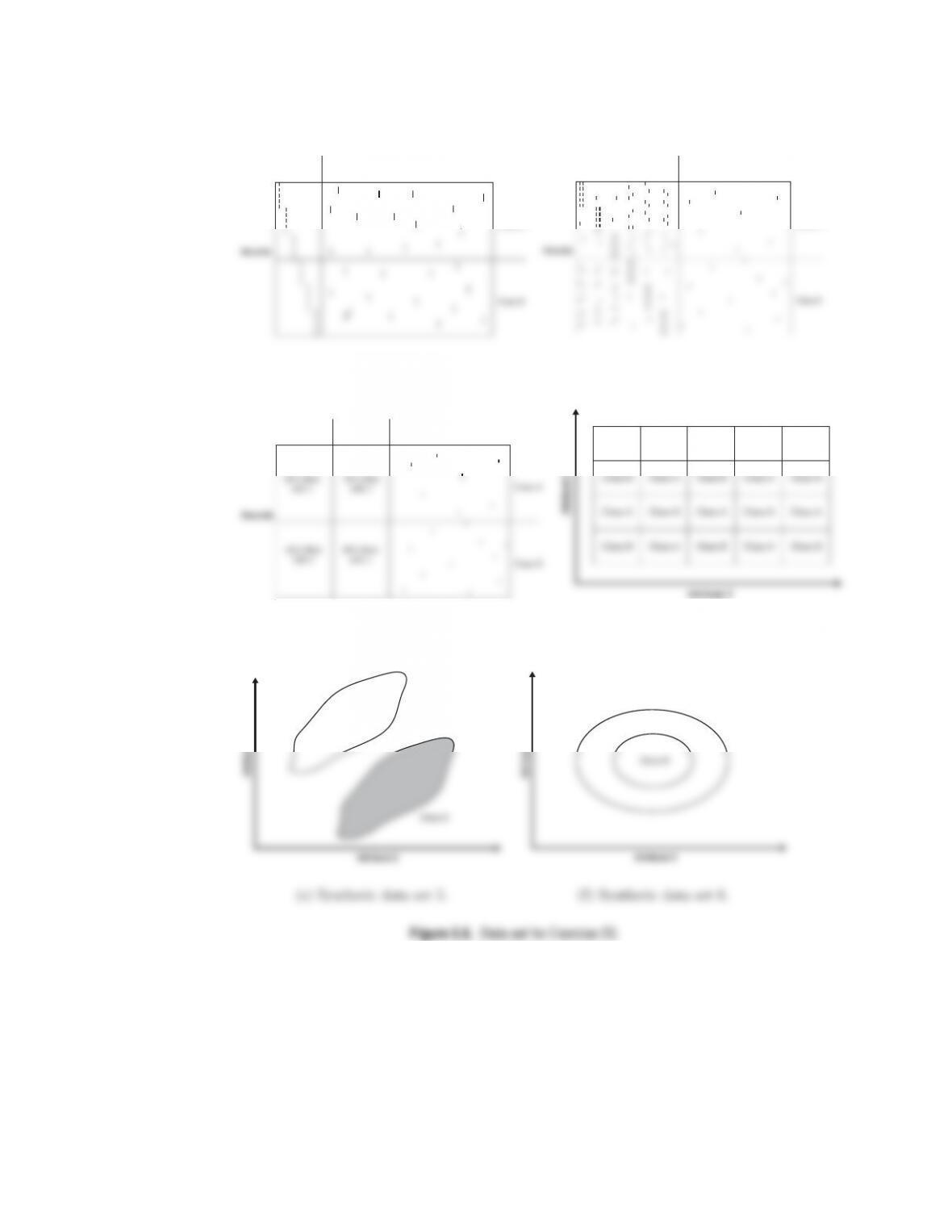
23. Given the data sets shown in Figures 5.6, explain how the decision tree, na¨ıve
Bayes, and k-nearest neighbor classifiers would perform on these data sets.
Answer:
(a) Both decision tree and NB will do well on this data set because the
distinguishing attributes have better discriminating power than noise
attributes in terms of entropy gain and conditional probability. k-NN
70 Chapter 5 Classification: Alternative Techniques
Distinguishing
Attributes Noise Attributes
Class A
Class B
Records
Attributes
(a) Synthetic data set 1.
Distinguishing Attributes Noise Attributes
Class A
Class B
Records
Attributes
(b) Synthetic data set 2.
Distinguishing
Attribute set 1 Noise Attributes
Attributes
Distinguishing
Attribute set 2
(c) Synthetic data set 3.
Class A Class B Class A Class B Class A
Attribute X
(d) Synthetic data set 4
Attribute X
Attribute Y
Class A
Class B
Attribute X
Attribute Y
Class A
Class B