4
Classification: Basic
Concepts, Decision
Trees, and Model
Evaluation
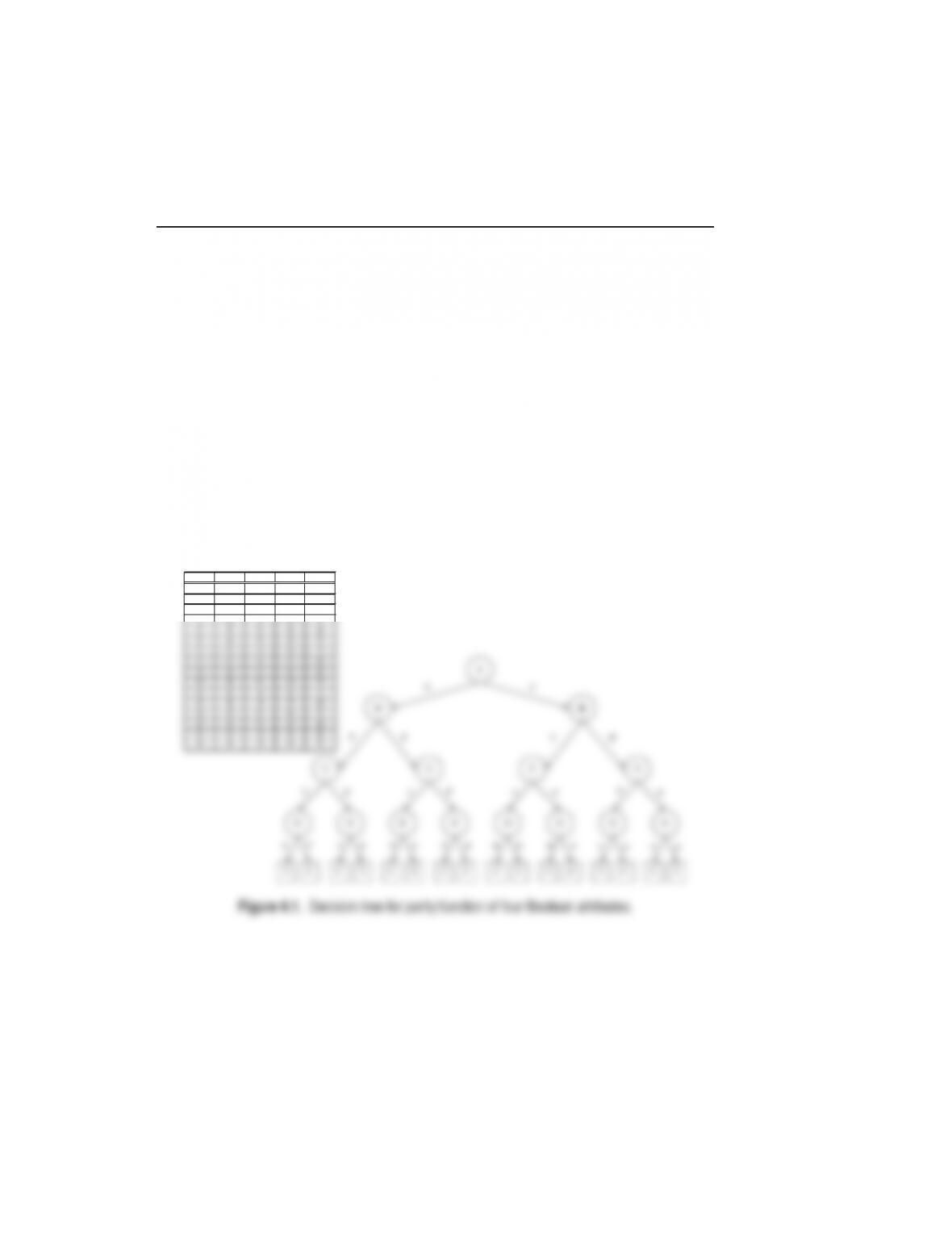
1. Draw the full decision tree for the parity function of four Boolean attributes,
A,B,C,andD. Is it possible to simplify the tree?
A B C D Class
TTTTT
TTTFF
TTFTF
26 Chapter 4 Classification
2. Consider the training examples shown in Table 4.1 for a binary classification
problem.
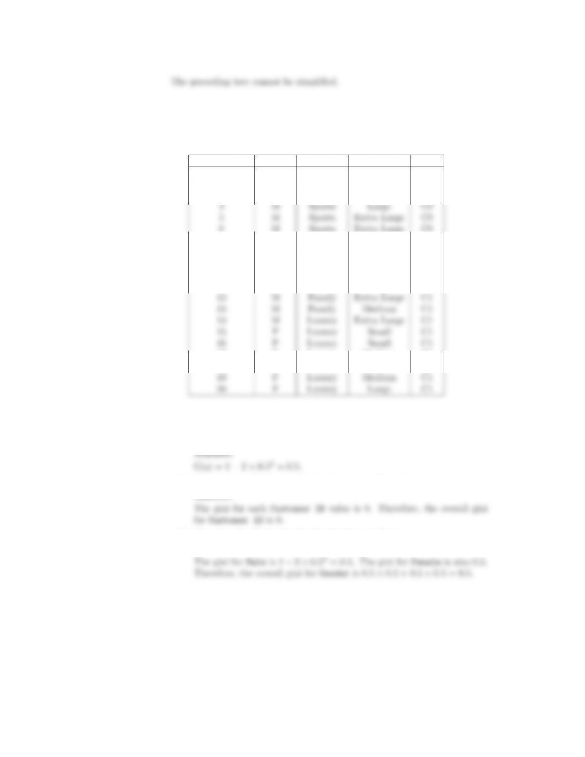
Table 4.1. Data set for Exercise 2.
Customer ID Gender Car Type Shirt Size Class
1 M Family Small C0
2 M Sports Medium C0
3 M Sports Medium C0
7 F Sports Small C0
8 F Sports Small C0
9 F Sports Medium C0
10 FLuxury Large C0
11 MFamily Large C1
17 FLuxury Medium C1
18 FLuxury Medium C1
(a) Compute the Gini index for the overall collection of training examples.
(b) Compute the Gini index for the Customer ID attribute.
Answer:
(c) Compute the Gini index for the Gender attribute.
Answer:
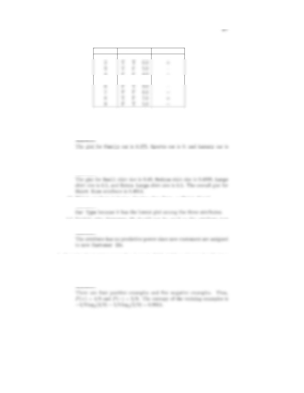
Table 4.2. Data set for Exercise 3.
Instance a1a2a3Target Class
1TT1.0 +
4FF4.0 +
5FT7.0 −
(d) Compute the Gini index for the Car Type attribute using multiway
split.
0.2188. The overall gini is 0.1625.
(e) Compute the Gini index for the Shirt Size attribute using multiway
split.
Answer:
(f) Which attribute is better, Gender,Car Type,orShirt Size?
Answer:
(g) Explain why Customer ID should not be used as the attribute test
condition even though it has the lowest Gini.
3. Consider the training examples shown in Table 4.2 for a binary classification
problem.
(a) What is the entropy of this collection of training examples with respect
to the positive class?
28 Chapter 4 Classification
(b) What are the information gains of a1and a2relative to these training
examples?
Answer:
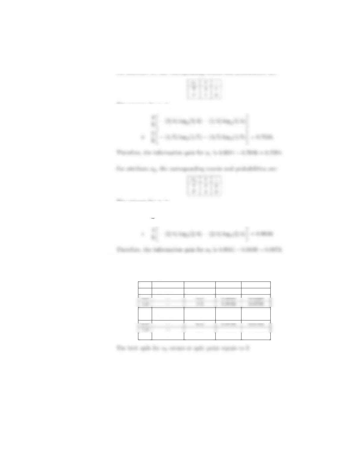
For attribute a1, the corresponding counts and probabilities are:
The entropy for a1is
The entropy for a2is
5
9−(2/5) log2(2/5) −(3/5) log2(3/5)
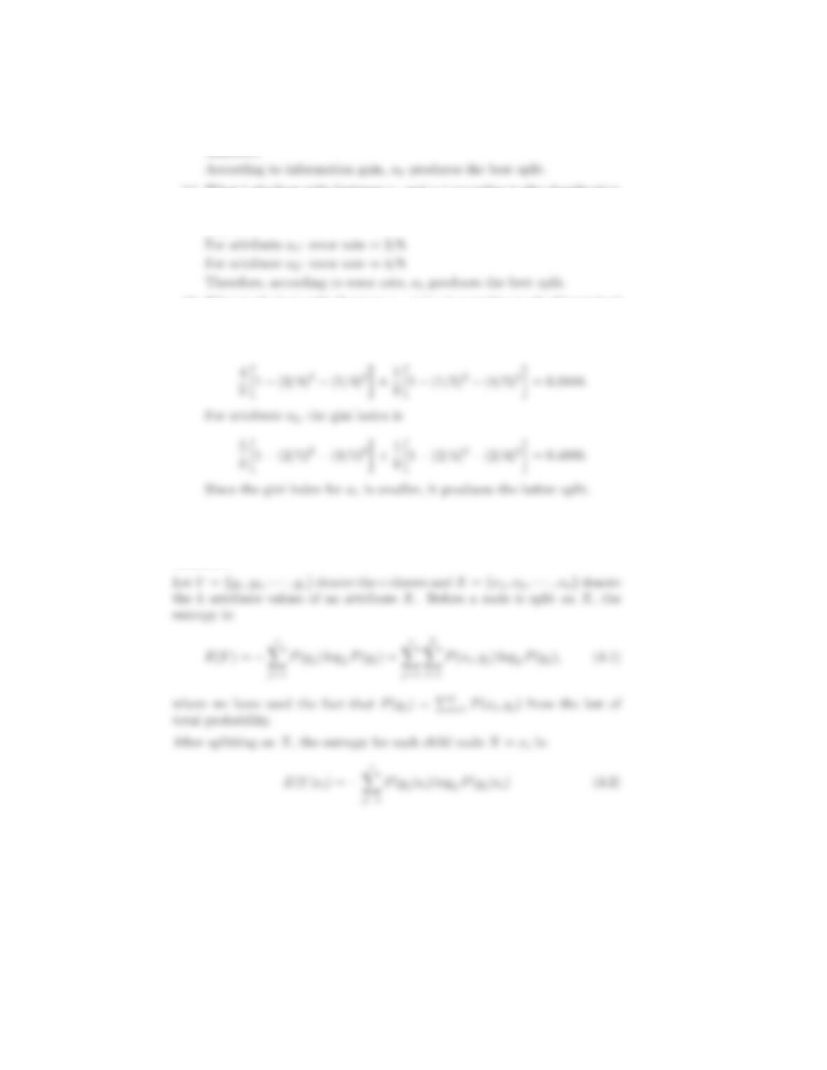
(c) For a3, which is a continuous attribute, compute the information gain
for every possible split.
Answer:
a3Class label Split point Entropy Info Gain
1.0 +2.0 0.8484 0.1427
5.0 –
5.0 –5.5 0.9839 0.0072
7.0 –7.5 0.8889 0.1022
29
(d) What is the best split (among a1,a2,anda3) according to the infor-
mation gain?
Answer:
(e) What is the best split (between a1and a2) according to the classification
error rate?
Answer:
(f) What is the best split (between a1and a2) according to the Gini index?
Answer:
For attribute a1, the gini index is
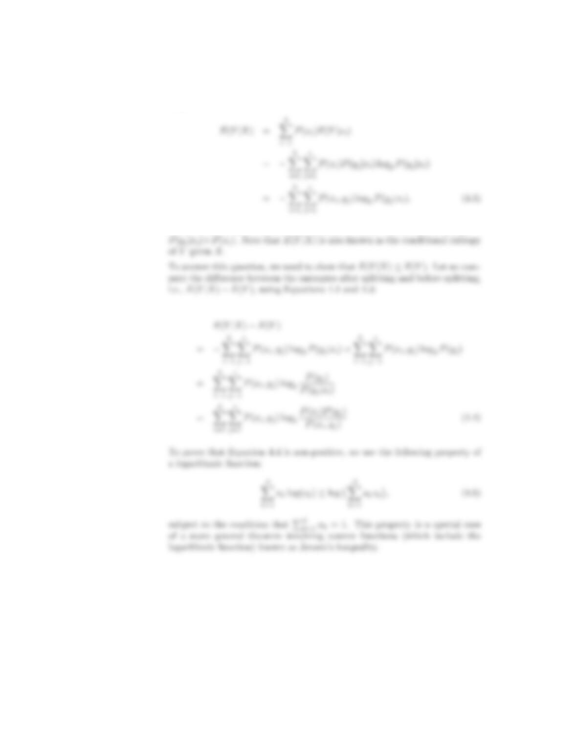
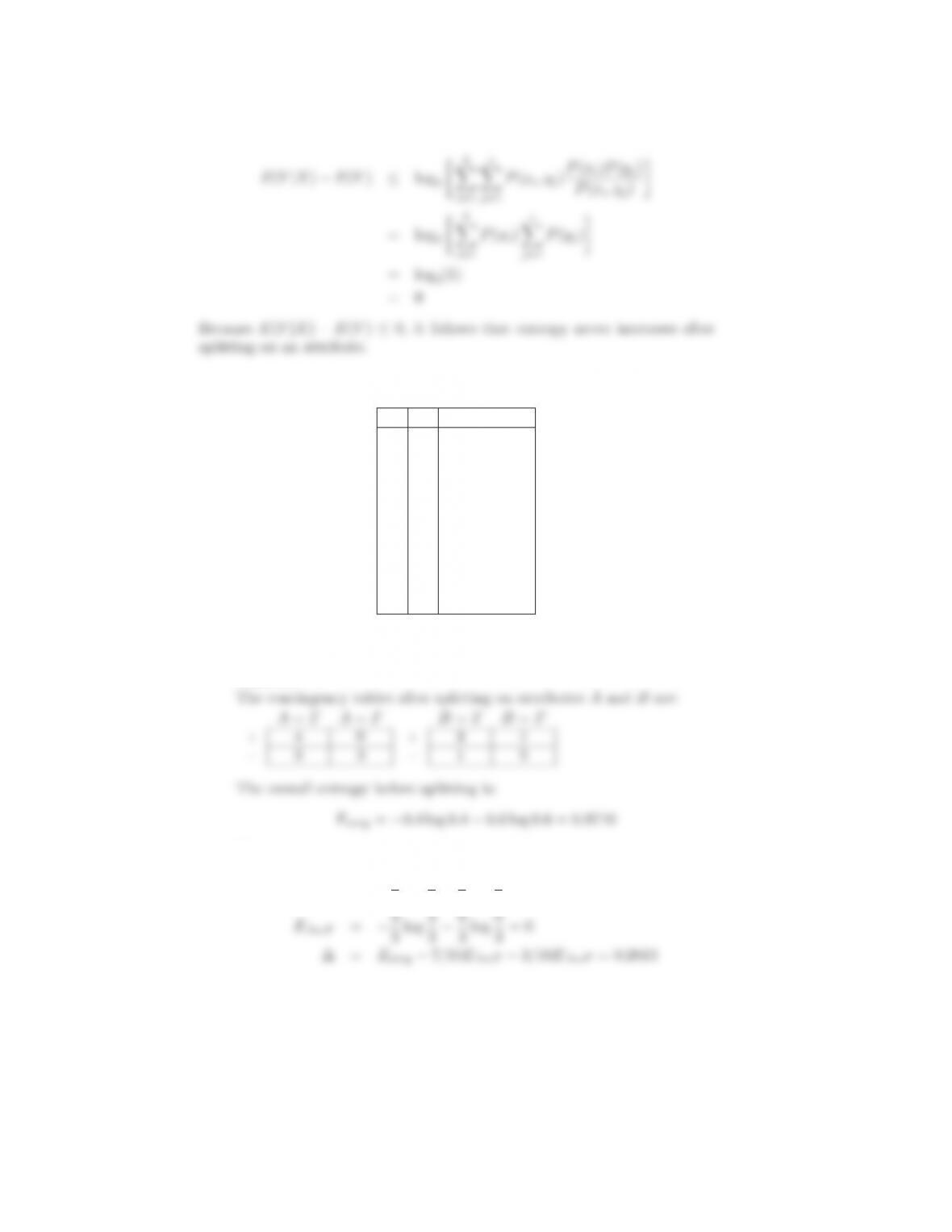
4. Show that the entropy of a node never increases after splitting it into smaller
successor nodes.
Answer:
j=1
30 Chapter 4 Classification
where P(yj|xi) is the fraction of examples with X=xithat belong to class
yj. The entropy after splitting on Xis given by the weighted entropy of the
children nodes:
k
i=1
j=1
where we have used a known fact from probability theory that P(xi,y
j)=
31
By applying Jensen’s inequality, Equation 4.4 can be bounded as follows:
c
5. Consider the following data set for a binary class problem.
A B Class Label
T F +
T T +
T T +
T F −
T T +
F F −
F F −
F F −
T T −
T F −
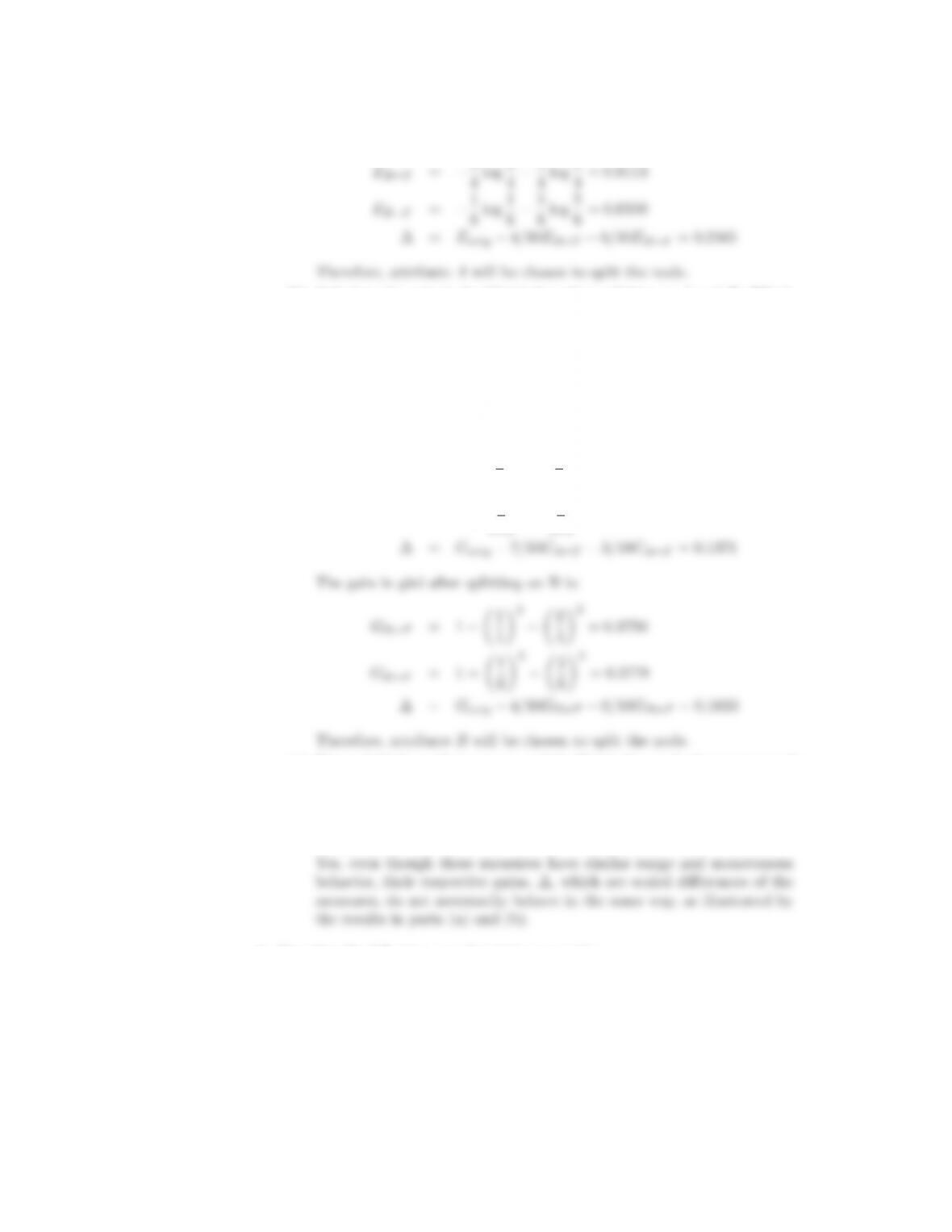
(a) Calculate the information gain when splitting on Aand B.Which
attribute would the decision tree induction algorithm choose?
Answer:
The information gain after splitting on A is:
EA=T=−4
7log 4
7−3
7log 3
7=0.9852
32 Chapter 4 Classification
The information gain after splitting on B is:
(b) Calculate the gain in the Gini index when splitting on Aand B.Which
attribute would the decision tree induction algorithm choose?
Answer:
The overall gini before splitting is:
Gorig =1−0.42−0.62=0.48
The gain in gini after splitting on A is:
GA=T=1−4
72
−3
72
=0.4898
GA=F=1=
3
32
−0
32
=0
(c) Figure 4.13 shows that entropy and the Gini index are both monotonously
increasing on the range [0, 0.5] and they are both monotonously decreas-
ing on the range [0.5, 1]. Is it possible that information gain and the
gain in the Gini index favor different attributes? Explain.
Answer:
6. Consider the following set of training examples.
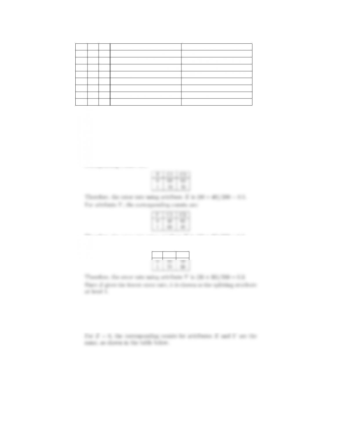
33
X Y Z No. of Class C1 Examples No. of Class C2 Examples
0 0 0 5 40
0 0 1 0 15
0 1 0 10 5
0 1 1 45 0
1 0 0 10 5
1 0 1 25 0
1 1 0 5 20
1 1 1 0 15
(a) Compute a two-level decision tree using the greedy approach described
in this chapter. Use the classification error rate as the criterion for
splitting. What is the overall error rate of the induced tree?
Answer:
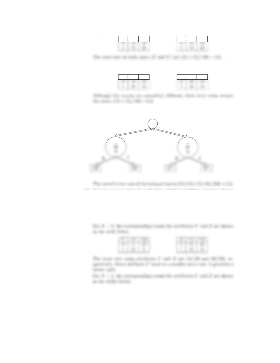
Splitting Attribute at Level 1.
To determine the test condition at the root node, we need to com-
pute the error rates for attributes X,Y,andZ. For attribute X,the
corresponding counts are:
Therefore, the error rate using attribute Yis (40 + 40)/200 = 0.4.
For attribute Z, the corresponding counts are:
ZC1 C2
Splitting Attribute at Level 2.
After splitting on attribute Z, the subsequent test condition may in-
volve either attribute Xor Y. This depends on the training examples
distributed to the Z=0andZ= 1 child nodes.
34 Chapter 4 Classification
XC1 C2 YC1 C2
For Z= 1, the corresponding counts for attributes Xand Yare shown
in the tables below.
XC1 C2 YC1 C2
The corresponding two-level decision tree is shown below.
Z
01
(b) Repeat part (a) using Xas the first splitting attribute and then choose
the best remaining attribute for splitting at each of the two successor
nodes. What is the error rate of the induced tree?
Answer:
After choosing attribute Xto be the first splitting attribute, the sub-
sequent test condition may involve either attribute Yor attribute Z.
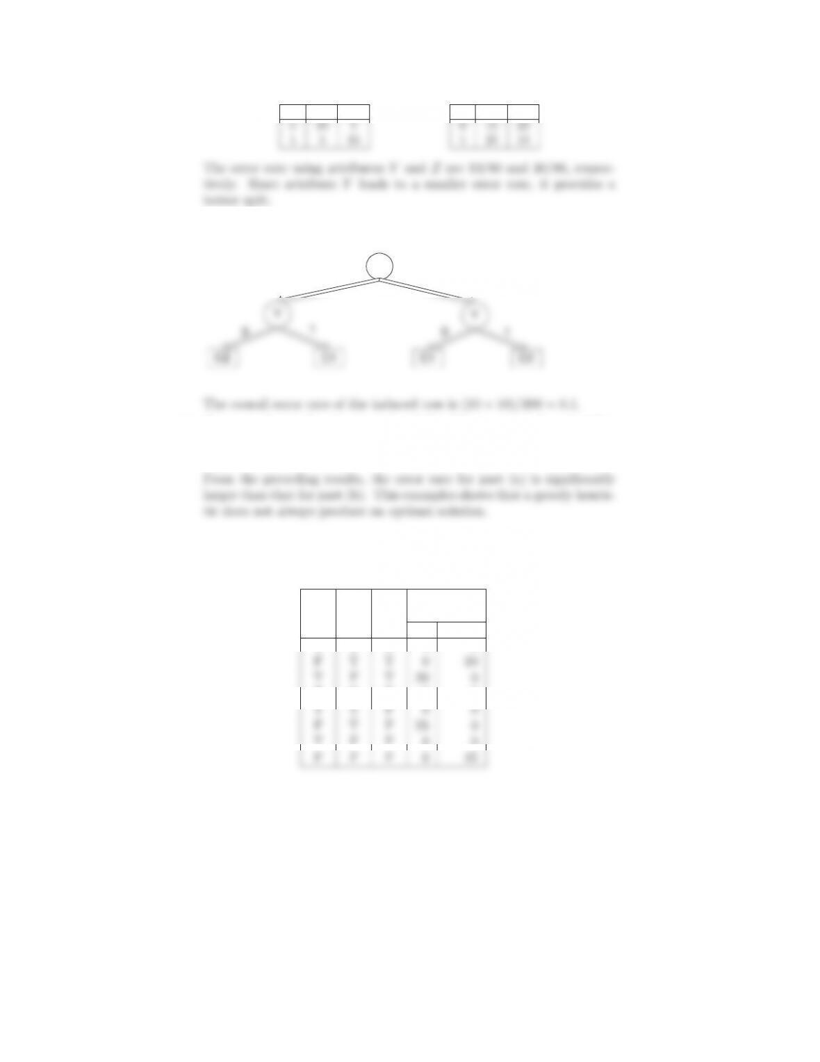
35
YC1 C2 ZC1 C2
The corresponding two-level decision tree is shown below.
X
01
YY
(c) Compare the results of parts (a) and (b). Comment on the suitability
of the greedy heuristic used for splitting attribute selection.
Answer:
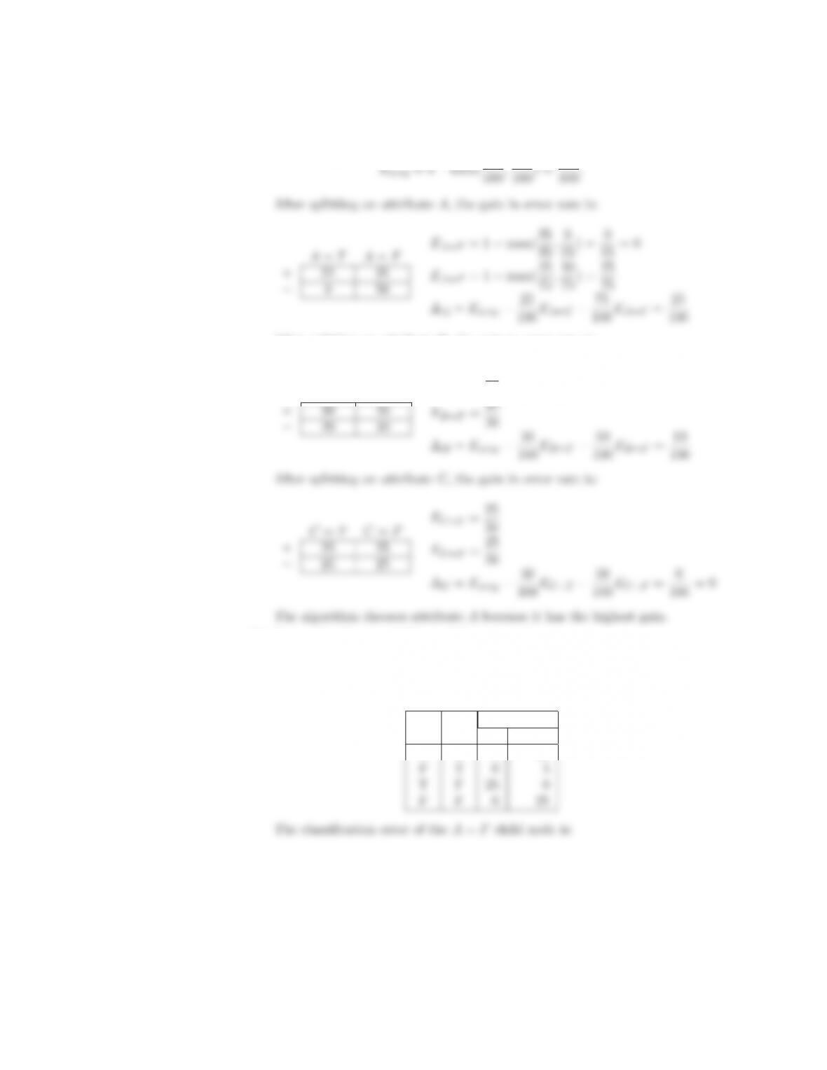
7. The following table summarizes a data set with three attributes A,B,Cand
two class labels +, −. Build a two-level decision tree.
A B C
Number of
Instances
+−
T T T 5 0
F F T 0 5
T F F 0 0
(a) According to the classification error rate, which attribute would be
chosen as the first splitting attribute? For each attribute, show the
contingency table and the gains in classification error rate.
36 Chapter 4 Classification
Answer:
The error rate for the data without partitioning on any attribute is
After splitting on attribute B, the gain in error rate is:
B=TB=F
EB=T=20
50
(b) Repeat for the two children of the root node.
Answer:
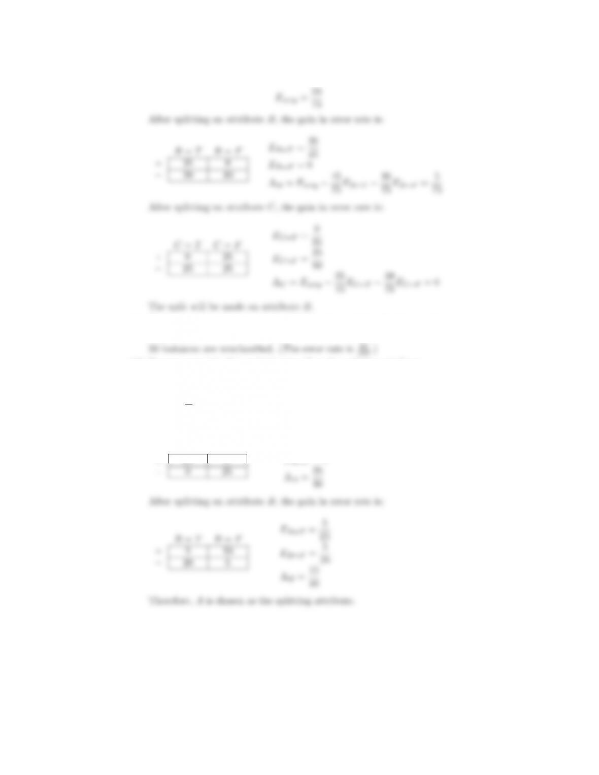
Because the A=Tchild node is pure, no further splitting is needed.
For the A=Fchild node, the distribution of training instances is:
B C Class label
+−
T T 0 20
37
(c) How many instances are misclassified by the resulting decision tree?
Answer:
(d) Repeat parts (a), (b), and (c) using Cas the splitting attribute.
Answer:
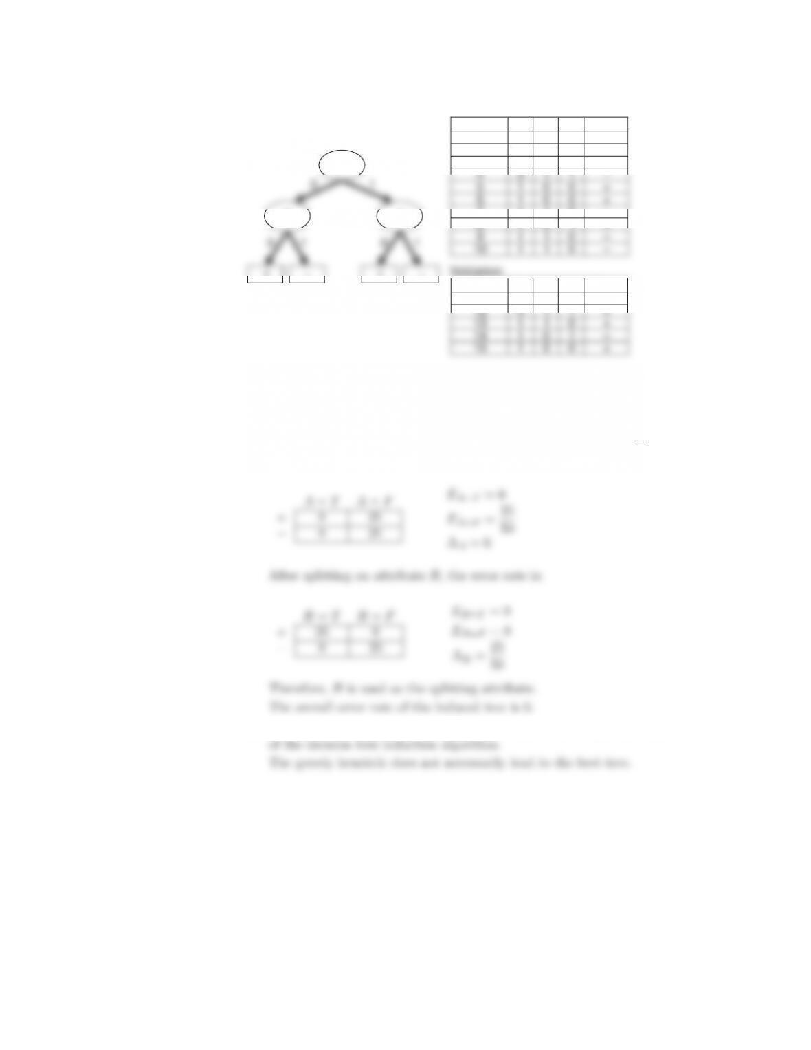
For the C=Tchild node, the error rate before splitting is:
Eorig =25
50 .
After splitting on attribute A, the gain in error rate is:
A=TA=F
+25 0
EA=T=0
EA=F=0
38 Chapter 4 Classification
+_+_
BC
A
Instance
1
2
3
7
8
0
0
0
1
1
0
0
1
1
0
0
1
0
0
1
ABC
+
+
+
–
+
Class
Training:
Instance
11
0
0
0
ABC
+
Class
Validation:
Figure 4.2. Decision tree and data sets for Exercise 8.
For the C=Fchild, the error rate before splitting is: Eorig =25
50 .
After splitting on attribute A, the error rate is:
EA=T=0
(e) Use the results in parts (c) and (d) to conclude about the greedy nature
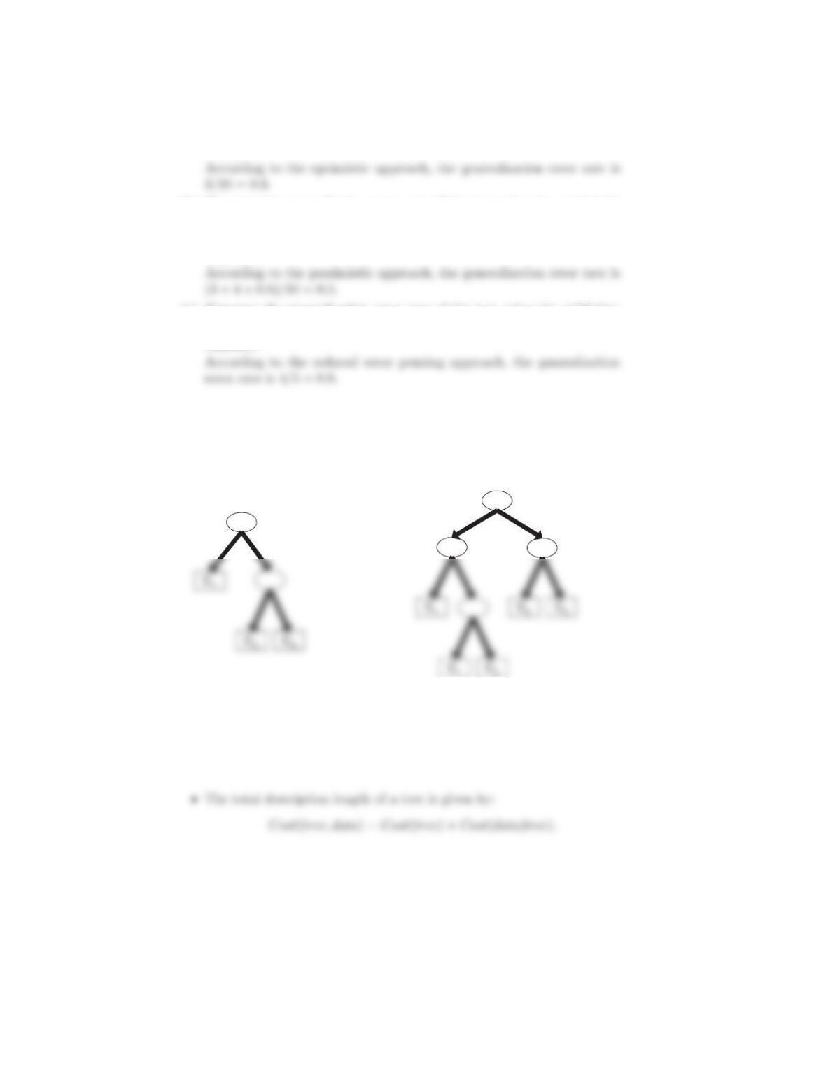
8. Consider the decision tree shown in Figure 4.2.
39
(a) Compute the generalization error rate of the tree using the optimistic
approach.
Answer:
(b) Compute the generalization error rate of the tree using the pessimistic
approach. (For simplicity, use the strategy of adding a factor of 0.5 to
each leaf node.)
Answer:
(c) Compute the generalization error rate of the tree using the validation
set shown above. This approach is known as reduced error pruning.
Answer:
9. Consider the decision trees shown in Figure 4.3. Assume they are generated
from a data set that contains 16 binary attributes and 3 classes, C1,C2,and
C3. Compute the total description length of each decision tree according to
the minimum description length principle.
(a) Decision tree with 7 errors (b) Decision tree with 4 errors
C1
Figure 4.3. Decision trees for Exercise 9.
40 Chapter 4 Classification
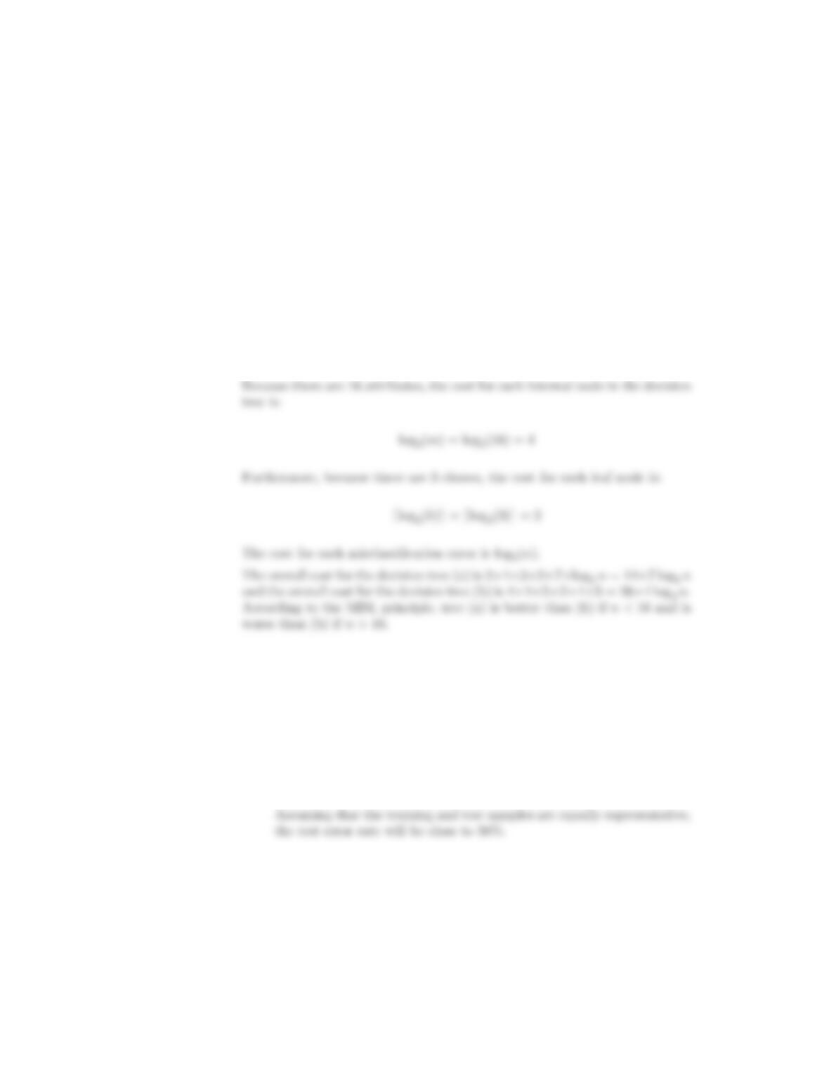
•Each internal node of the tree is encoded by the ID of the splitting
attribute. If there are mattributes, the cost of encoding each attribute
is log2mbits.
•Each leaf is encoded using the ID of the class it is associated with. If
there are kclasses, the cost of encoding a class is log2kbits.
•Cost(tree) is the cost of encoding all the nodes in the tree. To simplify
the computation, you can assume that the total cost of the tree is
obtained by adding up the costs of encoding each internal node and
each leaf node.
•Cost(data|tree) is encoded using the classification errors the tree com-
mits on the training set. Each error is encoded by log2nbits, where n
is the total number of training instances.
Which decision tree is better, according to the MDL principle?
Answer:
10. While the .632 bootstrap approach is useful for obtaining a reliable estimate
of model accuracy, it has a known limitation. Consider a two-class problem,
where there are equal number of positive and negative examples in the data.
Suppose the class labels for the examples are generated randomly. The clas-
sifier used is an unpruned decision tree (i.e., a perfect memorizer). Determine
the accuracy of the classifier using each of the following methods.
(a) The holdout method, where two-thirds of the data are used for training
and the remaining one-third are used for testing.
Answer:
41
(b) Ten-fold cross-validation.
Answer:
(c) The .632 bootstrap method.
Answer:
(d) From the results in parts (a), (b), and (c), which method provides a
more reliable evaluation of the classifier’s accuracy?
Answer:
11. Consider the following approach for testing whether a classifier A beats an-
other classifier B. Let Nbethesizeofagivendataset,pAbe the accuracy
of classifier A, pBbe the accuracy of classifier B,andp=(pA+pB)/2
be the average accuracy for both classifiers. To test whether classifier A is
significantly better than B, the following Z-statistic is used:
Z=pA−pB
2p(1−p)
N
.
Classifier A is assumed to be better than classifier B if Z >1.96.
Table 4.3 compares the accuracies of three different classifiers, decision tree
Table 4.3. Comparing the accuracy of various classification methods.
Data Set Size Decision na¨ıve Support vector
(N)Tree (%) Bayes (%) machine (%)
Anneal 898 92.09 79.62 87.19
Cleve 303 76.24 83.50 84.49
Credit 690 85.80 77.54 85.07
Diabetes 768 72.40 75.91 76.82
Ionosphere 351 89.17 82.34 88.89
Iris 150 94.67 95.33 96.00
Labor 57 78.95 94.74 92.98
Led7 3200 73.34 73.16 73.56
Lymphography 148 77.03 83.11 86.49
Pima 768 74.35 76.04 76.95
Zoo 101 93.07 93.07 96.04
Answer:
A summary of the relative performance of the classifiers is given below:
win-loss-draw Decision tree Na¨ıve Bayes Support vector
machine
Decision tree 0-0-23 9-3-11 2 – 7- 14
12. Let Xbe a binomial random variable with mean Np and variance Np(1 −p).
Show that the ratio X/N also has a binomial distribution with mean pand
variance p(1 −p)/N .

43