9.4. Hypothesis Tests of Variances
Problem 9-39.
X: n = 9; Y: n = 6
:
22
0
H
yx
VV
Problem 9-40.
S = 4095; Vo = 3500; n = 58, Ha: V<3500
Problem 9-41.
n = 58; S = 4095; D = 1%; Ho: V = 3500; HA: V > 3500
Problem 9-42.
4;22.13
1
)305.3)(15(
;305.3 22
XF
S
9-13
Problem 9-43.
096.0
1
)024.0)(15(
;024.0 22
F
S
Problem 9-44.
Level of significance = 0.01
Ho: S2 = 52
Problem 9-45.
Level of significance = 0.05
Problem 9-46.
݉݁ܽ݊ ൌͻ͵ͺ ͻͷͶ ͻͶ ͻͳ ͻͷͳ ͻͶͶ
ൌ ͻͶͻǤͳ݉ݒ
ݒܽݎ݅ܽ݊ܿ݁ ൌ ሾሺͻ͵ͺ െ ͻͶͻǤͳሻଶሺͻͷͶ െ ͻͶͻǤͳሻଶ
9-14
Problem 9-47.
Level of significance = 0.05
Ho: S2 = 52
Problem 9-48.
From Problem 9-35:
nX = 9; X: 1.74, 1.62, 1.59, 1.70, 1.73, 1.60, 1.56, 1.66, 1.71
ny = 6; Y: 1.46, 1.53, 1.49, 1.45, 1.51, 1.50
Problem 9-49.
Let A be wetlands with island and B be wetlands without island,
ܪǣߪଶൌߪ
ଶ
Problem 9-50.
B
AA
B
Ao
H
H
!
:
:
22
22
VV
VV
Problem 9-51.
H
o:VV VV
1
2
2
2
1
2
2
2
z;:HA
Problem 9-52.
:
22
H
yxo
VV
Problem 9-53.
9.5. Tests of Distributions
Problem 9-54.
Since n = 58, approximately eight cells are needed. For equal probabilities, the cumulative z
Cell P z x
j O
j E
j (O
j
E
j
)2/E
j
1 0.125 -1.150 3873 3 7.25 2.49
2 0.250 -.0.675 5834 11 7.25 1.94
The expected frequencies (Ej) are n/8 = 58/8 = 7.25. Since n, x, and S were used to compute F2,
Problem 9-55.
Converting the data to base 10 logs, the mean and standard deviation are 3.8894 and 0.2031.
Using a cell width of 0.5(standard deviation), produces the following:
Cell
Upper
Cell
bound
Oj
z
6p
P
Ej
Oj
Ej
(O
j
E
j
)2/E
j
1 3.585 3 -1.5 0.0668 .0668 3.9
2 3.686 6 -1.0 0.1587 .0919 5.3 9 9.2 0.004
Sum
58
1.000
58
58
2.912
Cells 1 and 8 were combined with the adjacent cells because the initial Ej < 5. Thus, there are 6
cells and 3 degrees of freedom. For D = 5%, FD
2 = 7.815. Therefore, accept Ho that the data are
Problem 9-56.
Cell
Upper
Cell
bound
Oj
z
6p
P
Ej
Ej
Oj
(O
j
E
j
)2/E
j
1 3.585 3 -.086 0.1949 0.1949 11.3 11.3 3 6.10
2 3.686 6 -0.46 0.3228 0.1279 7.4 7.4 6 0.26
Problem 9-57.
Cell
Upper
Cell
bound
Oj
6p
Pj
Ej
Ej
Oj
(Ej-Oj)2/Ej
1 0.351 22 0.1400 0.1400 5.2 5.2 22 54.28
2 1.014 7 0.4056 0.2656 9.8 9.8 7 0.80
Problem 9-58.
XS 8620 4128,
HQ N
nQ Q
nn
08620 4128:~( , )PV
HQ N
An Q Q
nn
:( , )z PV8620 4128
Range for
Annual max
discharge
qiP
V
= zi
CDF
=PZ z
i
()
Expected
prob.
Expected
frequenc
y
Ei
Observed
frequenc
y
Oi
()OE
E
ii
i
2
0 4319 -1.04 0.1492 0.1492 8.6536 6 0.8137
4319 8137 -0.12 0.4522 0.3030 17.5740 29 7.4288
9-18
Problem 9-59.
Using a cell width of 1000, the following table can be constructed:
Cell
Upper
Cell
bound
Oj
6O
j
6POj
z
6PE
j
|6PO
j
–6PE
j
|
1
2
4000
5000
3
6
3
9
.0517
.1552
-1.12
-0.88
.1314
.1894
.0797
.0342
3 6000 6 15 .2586 -0.63 .2643 .0057
4 7000 8 23 .3966 -0.39 .3483 .0487
5 8000 7 30 .5172 -.015 .4404 .0768
6 9000 9 39 .6724 0.09 .5359 .1365
Problem 9-60.
The mean and standard deviation are x = 3.8894, and S = 0.2031. The following table can be
constructed for the test:
Cell
Upper
Cell
bound
Oj
6O
j
6PO
j
zj
6PE
j
|6PO
j
–6PE
j
|
1 3.5 3 3 .052 -1.92 .027 0.025
2 3.6 0 3 .052 -1.42 0.78 0.026
3 3.7 6 9 .155 -0.93 .176 0.021
4 3.8 9 18 .310 -0.44 .330 0.020
Problem 9-61.
mean = 45.19 sd = 2.216
9-19
x rank i/n z Sp diff
41.6 1 0.111 -1.620 0.530 0.058
42.9 2 0.222 -1.033 0.151 0.071
Problem 9-62.
z = (x-20)/1.5 p(x) = i/12 D0.20 = 0.295 D0.05 = 0.375
Hence, accept Ho, the assumed distribution is acceptable.
i x z F(z) p(x) F(z)-p(x)
1 16.7 -2.200 0.0139 0.0833 0.0694
2 17.2 -1.867 0.0309 0.1667 0.1358
3 17.9 -1.400 0.0808 0.2500 0.1692
Problem 9-63.
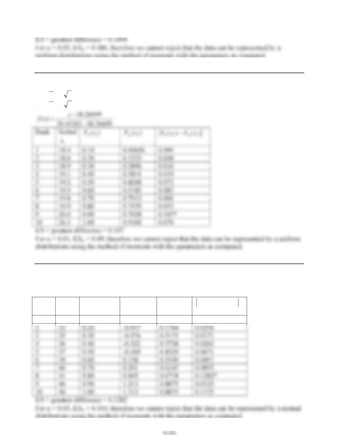
Uniform parameters:
83.143 SX
D
Problem 9-64.
Uniform parameters:
26699.183 SX
D
45301.203 SX
E
Problem 9-65.
Normal distribution parameters:
1.38
P
512.6
V
Rank Sorted
i
x
)( iS xF z )( iX xF )()( iXiS xFxF
1 29 0.10 -1.397 0.0812 0.0188
9-21
Problem 9-66.
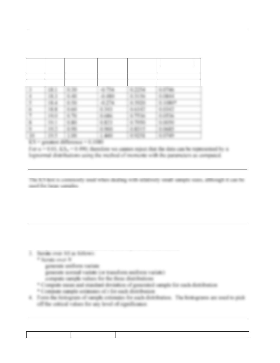
Lognormal distribution parameters:
269.1
Y
P
01458.0
Y
V
Rank Sorted
i
x
)( iS xF z )( iX xF )()( iXiS xFxF
1 17.6 0.10 -1.578 0.0573 0.0427
2 17.9 0.20 -1.097 0.1363 0.0637
Problem 9-67.
9.7. Simulation of Hypothesis Test Assumptions
Problem 9-68.
The procedure is as follows:
1. Input seed, sample size (N), number of samples simulated (NS)
2. Set parameters of normal, uniform, and exponential distributions
Problem 9-69.
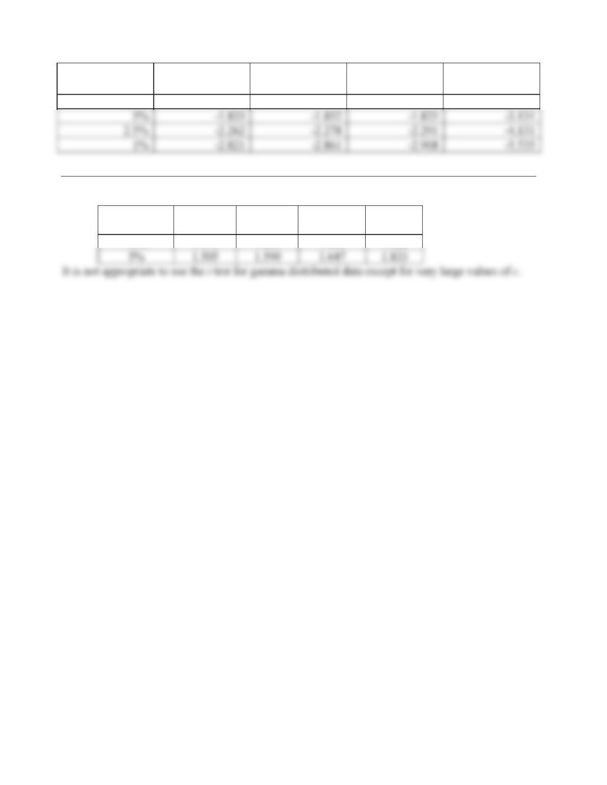
The following is the result of simulation:
Critical Values for
9-22
Significance
Level (D)
t
D
,
Q
Normal Uniform Exponential
10% -1.383 -1.398 -1.366 -2.194
Problem 9-70.
Using simulation, the following results can be obtained:
Significance
Level (D)
t for c = 3 t for c = 6 t for c = 10 t9
10% 1.175 1.224 1.249 1.383