7-1
CHAPTER 7. SIMULATION
CHAPTER 7. SIMULATION …………………………………..………………………………………………………….1
7.1. Introduction ………………………………………………………………………………………………………………1
7.2. Monte Carlo Simulation ……………………………..………………………………………………………………1
7.3. Random Numbers ………………………………………………………………………………………………………1
7.4. Generation of Random Variables ………………………………………………………………………………...4
7.5. Generation of Selected Discrete Random Variables ……………………………………………………….5
7.6. Generation of Selected Continuous Random Variables …….…………………………………………….9
7.9. Simulation Projects ………………………………………………………………………………………..…………11
The following table provides a summary of the problems with their appropriate sections:
Section Problems
7.1
7.1. Introduction
7.2. Monte Carlo Simulation
7.3. Random Numbers
Problem 7-1.
7-2
16 25 0.961538
17 24 0.923077
18 17 0.653846
Problem 7-2.
i Ii U
i
0 3 0.008696
1 26 0.075362
2 187 0.542029
7-3
22 302 0.875362
23 49 0.142029
24 3 0.008696
25 26 0.075362
Problem 7-3.
seed = 3
a = 77
b = 345
c = 26
i Ii U
i
0 3 0.115385
1 -7014 -269.769
7-4
18 2.67E+54 1.03E+53
19 -2.5E+57 -9.7E+55
20 2.38E+60 9.15E+58
21 -2.2E+63 -8.6E+61
Problem 7-4.
Based on the results of Problems 7-1, 7-2 and 7-3, and parametric analysis, the following
7.4. Generation of Random Variables
Problem 7-5.
(a) To four significant digits, the range of uniform variates that represent 1 to 6 on a fair die
Problem 7-6.
x y
4,5 2
Problem 7-7.
7-5
Problem 7-8.
7.5. Generation of Selected Discrete Random Variables
Problem 7-9.
The Bernoulli distribution produces the following values:
uixu
ixu
ixu
ix
Problem 7-10.
Problem 7-11.
The binomial distribution produces the following values:
ui
x
0.47, 0.06, 0.02 2
Problem 7-12.
Ui Xi Ui Xi
0.17 0.35 2 0.43 0.35 2
Problem 7-13.
Ui Xi Ui Xi
0.05 0.37 0.23 3 0.69 0.93 0.77 0
7-7
Problem 7-14.
The following cumulative function can be used:
N
Entering FN(n) with the ui, the value of n is determined:
Hence, the geometric distribution id f(x) = 04(06)x-1
x 1 2 3 4 5 6
Problem 7-16.
(c)
Ui Xi Use Xi
0.76 3.2 3
Problem 7-17.
For O = 1.5, the following is the cumulative Poisson distribution:
x0 1 2 3 4 5 6 7
ixu
ixu
ixu
ix
0.43 1 0.48 1 0.85 3 0.54 1 0.34 1
0.53 1 0.87 3 0.81 3 0.71 2 0.89 3
Problem 7-18.
!
5.1
)(
5.1
x
e
xp x
x x! f(x) F(x) n/N
0 1 0.223 0.223 0.25
7-9
7.6. Generation of Selected Continuous Random Variables
Problem 7-19.
x 0 1 2 3 4 5 6 7 8
f(x) 0.0498 0.1494 0.2240 0.2240 0.1680 0.1008 0.0504 0.0216 0.0081
Problem 7-20.
!
2
)(
2
x
e
xf x
x 0 1 2 3 4 5 6
f(x) 0.135 0.271 0.271 0.180 0.090 0.036 0.012
Problem 7-21.
The transformation equation of Eq. 7-30 is: Xi = 4 + 6Ui
Problem 7-22.
7-10
Problem 7-23.
Ui 0.68 0.04 0.76 0.37
Problem 7-24.
U(2,4) 2.76 3.47 2.06 3.84
Problem 7-26.
Ui 0.55 0.38 0.82 0.27 0.64
Problem 7-27.
Ui 0.13 0.71 0.44 0.6 0.27
Problem 7-28.
1488.0
y
V
Ui 0.39 0.61 0.50 0.13 0.82
zi -0.27923 0.27923 0 -1.12636 0.91538
Problem 7-29.
Ui 0.03 0.82 0.37 0.54
Problem 7-30.
4.1/)(ln/)(ln uieuiexi
O
Problem 7-31.
The mean of the xi values is 0.84. Therefore 84.0
O
, and )84.0/(ln uiexi
7.9. Simulation Projects
Problem 7-32.
I u1 u2 u3 u4 Pi Li Ei Ai PL/AE
1 0.195578 0.358648 0.483826 0.096098 70.51923 19.63792 29730.6 0.934794 0.049829
2 0.97875 0.491353 0.862759 0.990389 188.1032 19.97832 33289.12 1.117061 0.101059
3 0.519326 0.788693 0.371827 0.82585 95.95361 20.80189 28893.07 1.046895 0.065988
4 0.509991 0.960403 0.926041 0.884171 95.19289 21.75538 34486.05 1.059805 0.056663
5 0.834911 0.325154 0.859806 0.649976 131.4214 19.54667 33244.81 1.019263 0.07581
6 0.875431 0.553239 0.363053 0.624435 139.6518 20.13385 28826.02 1.015858 0.096019
The mean change in length is 0.06883 in, and the variance is 0.000306 in2.
7-12
Problem 7-33.
Using different starting seeds as was used in Problem 7-32, the results are summarized as follows:
Simulation
Cycles (N)
Mean Variance Sample Variance =
Variance/N
Problem 7-34.
Using N = 20 cycles, a histogram is given by
0.0665
0.067
0.0675
0.0004
0.0005
0.0006
0.0007
0.00002
0.000025
0.00003
7-13
Using N = 100 cycles, a histogram is given by
Comparing the above two figures, it is clear that 20 cycles are not enough to obtain a histogram for
deformation. However, a sample size of 100 is adequate. Normal and lognormal distributions can
be statistically tested for their suitability as models.
Problem 7-35.
Using N = 1000 cycles, a histogram is given by
Normal and lognormal distributions can be statistically tested for their suitability as models.
0.3
0.35
0.4
0.15
0.2
0.25
0.2
0.25
7-14
Problem 7-36.
Based on a graphical examination of the charts in the solutions to Problems 7-34 and 7-35, the
chart of 7-35 looks more like a lognormal than a normal distribution due to its skewness toward
Problem 7-37.
The following are the results of 100 simulation cycles broken down in two tables:
i u1 u2 u3 u4 u5 As fy d
1 0.871985 0.977322 0.489352 0.133112 0.505368 0.278602 48005.34 19.94842
2 0.329495 0.18442 0.395248 0.937566 0.047866 0.238046 36405.4 19.71163
3 0.307341 0.606459 0.249966 0.128046 0.751591 0.236576 41080.41 19.31293
4 0.58675 0.686511 0.438765 0.324566 0.776754 0.254258 41943.94 19.82183
5 0.710565 0.672868 0.445144 0.969183 0.552727 0.26292 41791.39 19.83784
6 0.543178 0.763026 0.886868 0.14639 0.910975 0.251465 42864.28 21.22009
17 0.857307 0.825016 0.692051 0.843893 0.085844 0.276732 43738.61 20.48211
18 0.289161 0.058057 0.388671 0.350035 0.903888 0.235342 33714.81 19.69478
19 0.297137 0.393893 0.631225 0.46775 0.983959 0.235887 38923.25 20.31233
20 0.674276 0.271086 0.542622 0.30459 0.591919 0.260225 37561.87 20.08217
21 0.447981 0.832623 0.404972 0.438606 0.757529 0.245536 43858.33 19.73643
22 0.901944 0.201219 0.383264 0.24413 0.815598 0.282997 36650.9 19.68087
23 0.196896 0.929027 0.184725 0.397515 0.205284 0.228474 45874.34 19.09901
24 0.308842 0.351873 0.958285 0.529285 0.319741 0.236677 38478.92 21.77987
25 0.389207 0.6126 0.553143 0.627695 0.806932 0.241874 41144.41 20.10885
52 0.362783 0.098605 0.608235 0.685212 0.681069 0.2402 34841.83 20.25115
53 0.992896 0.447045 0.641851 0.83342 0.227457 0.31769 39467.48 20.34109
54 0.064147 0.194253 0.972409 0.244829 0.680838 0.213744 36550.69 21.9836
55 0.719089 0.388325 0.9518 0.836735 0.783915 0.26358 38865.25 21.70538
56 0.043022 0.73182 0.415403 0.882826 0.444998 0.20961 42473.31 19.76291
57 0.5407 0.421854 0.235997 0.939128 0.389734 0.251308 39211.39 19.2699
58 0.791507 0.604407 0.094333 0.653295 0.224409 0.269738 41059.09 18.70513
59 0.127921 0.518949 0.811912 0.002621 0.948818 0.222103 40190.07 20.87818
60 0.557581 0.213196 0.01027 0.068461 0.564387 0.252379 36818.48 17.79181
73 0.999621 0.486284 0.004859 0.935914 0.827439 0.348062 39862.45 17.554
74 0.491052 0.835756 0.175141 0.275629 0.167594 0.248203 43908.66 19.06418
75 0.149106 0.580013 0.519799 0.153222 0.007278 0.22424 40807.71 20.02466
76 0.693421 0.294566 0.144038 0.8087 0.453368 0.261626 37839.62 18.94234
77 0.736594 0.29685 0.573344 0.027587 0.147144 0.26497 37866.07 20.16045
78 0.309259 0.440479 0.158035 0.271376 0.390885 0.236705 39400.98 18.99901
79 0.092951 0.086974 0.383807 0.58277 0.594419 0.218009 34561.49 19.68227
80 0.999334 0.67523 0.641087 0.329381 0.060816 0.342618 41817.6 20.33901
81 0.482954 0.301028 0.605723 0.013735 0.106184 0.247701 37914.21 20.24454
7-16
94 0.648979 0.838636 0.455554 0.205294 0.405385 0.258436 43955.47 19.86392
95 0.499493 0.730458 0.036151 0.250302 0.426951 0.248728 42456.79 18.25939
96 0.297542 0.373868 0.964066 0.302768 0.696039 0.235915 38713.49 21.8549
97 0.009556 0.057234 0.305545 0.964386 0.44301 0.196907 33686.29 19.47387
98 0.011723 0.34468 0.313622 0.29565 0.794196 0.198431 38401.1 19.49618
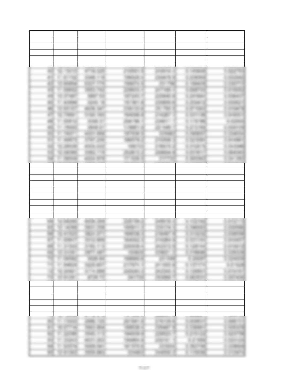
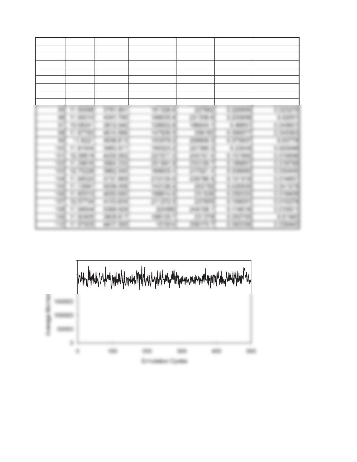
i b fc’ M=asfy(d-a/2) Average COV Sample COV
1 11.33292 3932.788 264437.4 264437.4 na na
2 12.9208 2820.079 169611.9 217024.6 0.308959 0.218467
3 11.31859 4487.315 186601.8 225519.6 0.24405 0.140903
4 11.72702 4560.575 210140.8 237289.1 0.1618 0.0809
14 12.53932 4075.087 202324.3 233380.9 0.188193 0.050297
15 12.03483 2736.372 203973.7 234205.6 0.18255 0.047134
16 11.54683 3569.874 169188.7 216813.1 0.310641 0.07766
17 12.60635 2992.174 245628.3 255032.9 0.05215 0.012648
18 11.76886 5078.098 155648.8 210043.1 0.366235 0.086322
19 11.95144 5996.436 185805.5 225121.5 0.246983 0.056662
20 11.69325 4107.136 195124.1 229780.8 0.213299 0.047695
21 11.9073 4504.117 211265.4 237851.4 0.158075 0.034495
34 12.26428 3484.211 193024.2 228730.8 0.220769 0.037862
35 12.01882 4110.372 263218.2 263827.8 0.003268 0.000552
36 10.5725 3768.839 254630.4 259533.9 0.02672 0.004453
37 13.1309 3478.172 190767.9 227602.6 0.228874 0.037627
38 12.46993 3931.314 209748.4 237092.9 0.163105 0.026459
55 12.58868 4582.493 221281.7 242859.5 0.125652 0.016943
56 12.71354 3816.345 174984.8 219711.1 0.28789 0.038471
57 12.9285 3710.735 188697.7 226567.6 0.23638 0.031309
58 12.23654 3375.992 205416.2 234926.8 0.177648 0.023326
59 10.32489 5420.491 185528 224982.7 0.248007 0.032288
60 11.10759 4050.284 164196.6 214317 0.33073 0.042697
61 11.7084 5308.245 144781.5 204609.5 0.413517 0.052945
62 12.95648 4153.04 224637.7 244537.6 0.115085 0.014616
63 10.74504 3570.364 245066.8 254752.1 0.053767 0.006774
74 11.64248 3240.822 205915 235176.2 0.17596 0.020455
75 11.38637 2417.711 181450.8 222944.1 0.263207 0.030392
76 12.52387 3832.365 186324.9 225381.2 0.245069 0.028111
77 10.8495 3186.696 200564.5 232501 0.194257 0.022138
78 11.63481 3712.938 176008.1 220222.7 0.283935 0.032149
7-18
86 12.35695 3111.534 204719 234578.2 0.180014 0.019411
87 12.19212 3099.845 231140.2 247788.8 0.095019 0.010187
88 12.69578 3451.589 192867.2 228652.3 0.221331 0.023594
89 12.7067 3450.949 226283.5 245360.4 0.109956 0.011655
90 12.84511 4032.479 212429.3 238433.4 0.154237 0.016258
91 11.07137 4570.388 229339.8 246888.6 0.100522 0.010538
92 12.54848 3467.241 194371.8 229404.6 0.215967 0.022516
93 12.01367 5890.574 247259.9 255848.6 0.047475 0.004923
94 11.50628 3740.676 223884 244160.7 0.117446 0.012114
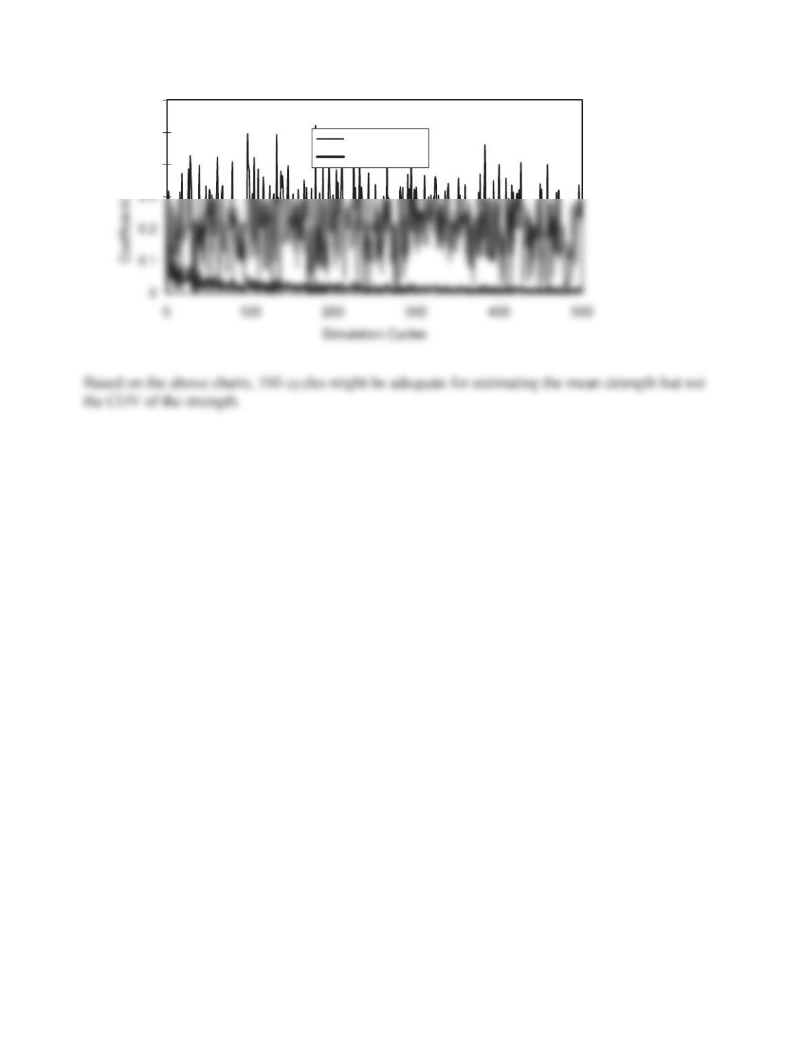
The effect of adding more simulation cycles on the results is studied in the following charts:
200000
250000
300000
7-19
0.4
0.5
0.6
COV
Sample COV