6-1
CHAPTER 6. MULTIPLE RANDOM VARIABLES
CHAPTER 6. MULTIPLE RANDOM VARIABLES ……………………………………………………………..1
6.1. Introduction ………………………………………………………………………………………………………………1
6.2. Joint Random Variables and Their Probability Distributions …………………………………………..1
6.3. Functions of Random Variables …………………………………………………………………………………..8
6.5. Multivariable Simulation …………………………………………………………………………………………..14
The following table provides a summary of the problems with their appropriate sections:
Section Problems
6.1. Introduction
None
6.2. Joint Random Variables and Their Probability Distributions
Problem 6-1.
X = Condition of Cargo
Y \ X ND D PD PY (y)
Problem 6-2.
X = Thermal Test
Y \ X A NA PA PY (y)
Y = A 0.80 0.02 0.00 0.82
Problem 6-3.
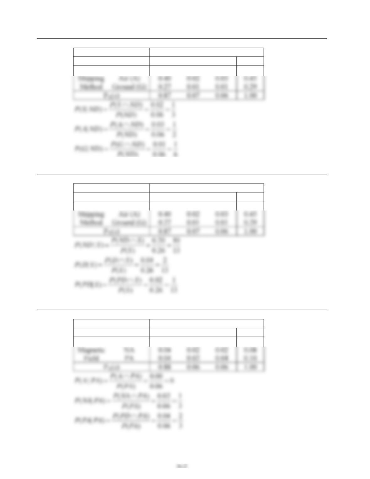
X = Condition of Cargo
Y \ X ND D PD PY (y)
Y = Sea (S) 0.20 0.04 0.02 0.26
Problem 6-4.
X = Condition of Cargo
Y \ X ND D PD PY (y)
Y = Sea (S) 0.20 0.04 0.02 0.26
Problem 6-5.
X = Thermal Test
Y \ X A NA PA PY (y)
Y = A 0.80 0.02 0.00 0.82
6-3
Problem 6-6.
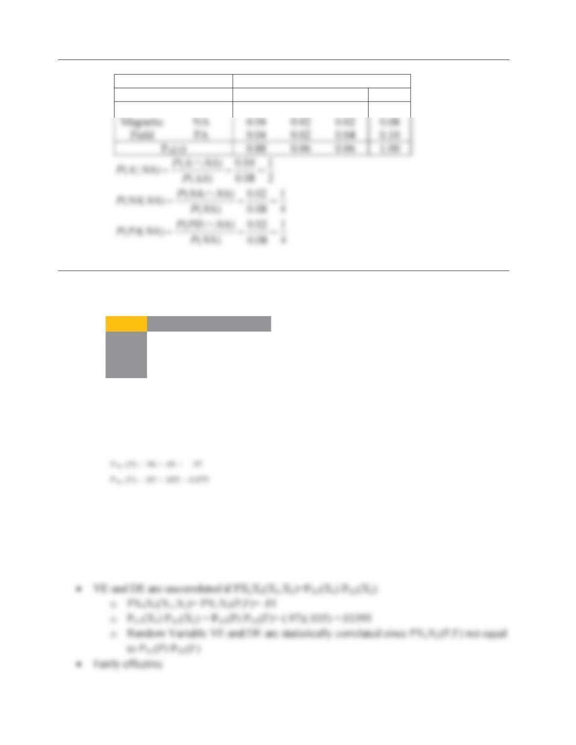
X = Thermal Test
Y \ X A NA PA PY (y)
Y = A 0.80 0.02 0.00 0.82
Problem 6-7.
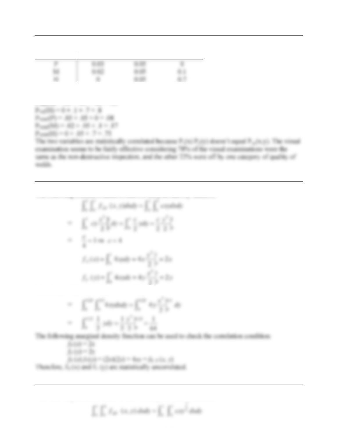
Joint Probability Mass Function:
n=1000 X
1
, VE
P F
X
2
, DE P 0.96 0.005
F 0.01 0.025
Marginal Prob Mass Functions of VE
Marginal Prob Mass Functions of DE
P
X
2
(P) = .96 + .005 = .965
P
X
2
(F) = .01 + .025 = .035
6-4
Problem 6-8.
The joint probability mass function (joint PMF):
P M H
The marginal probability mass function (marginal PMF):
PVE(P) = .03+.02+0 = .05
Problem 6-9.
The following condition needs to met for the joint density function:
Therefore, P
X
Y(.,.)0050025
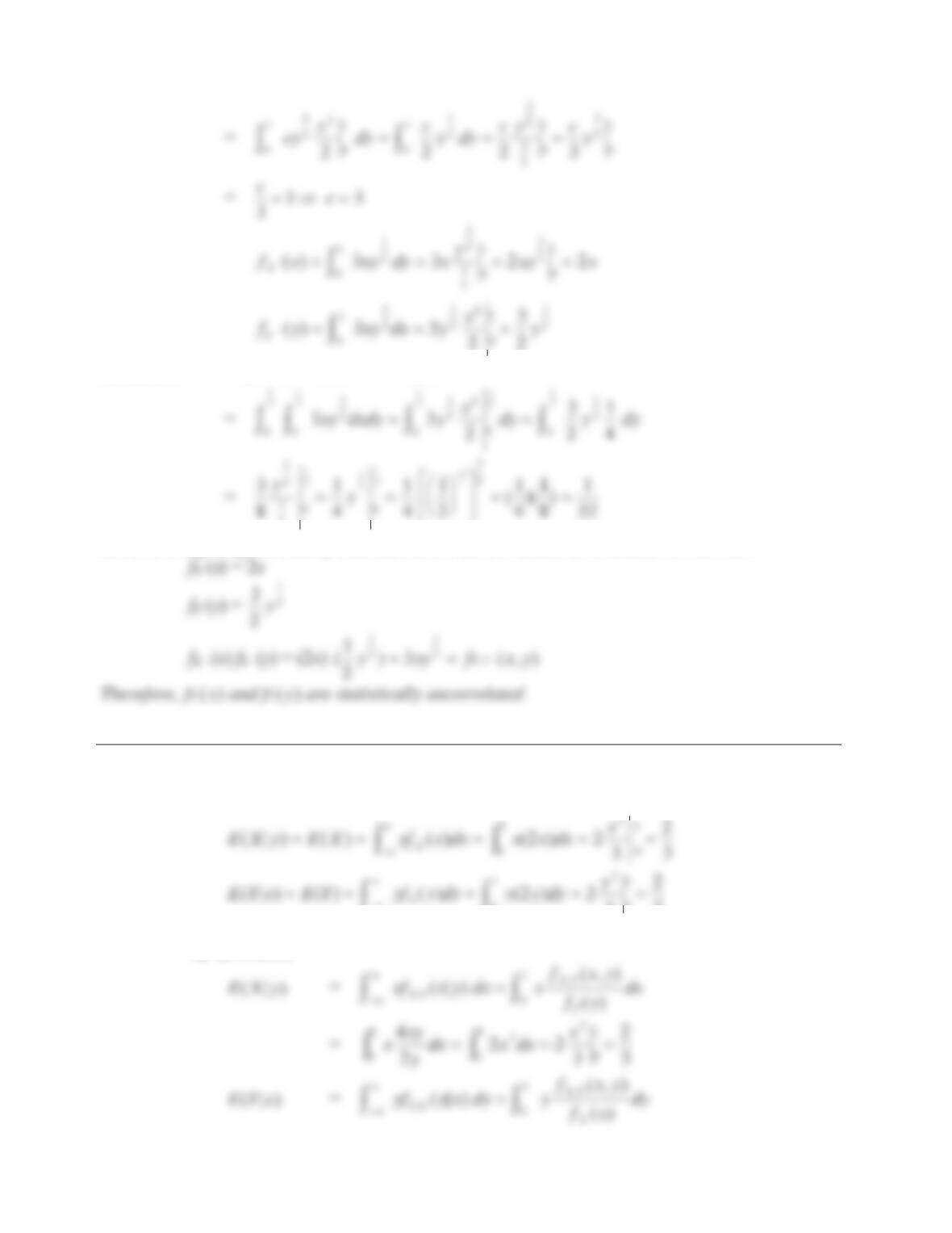
Problem 6-10.
The following condition needs to met for the joint density function:
6-5
Therefore, P
X
Y
(.,.)0050025
2
¬
«
¼
» ()()
The following marginal density function can be used to check the correlation condition:
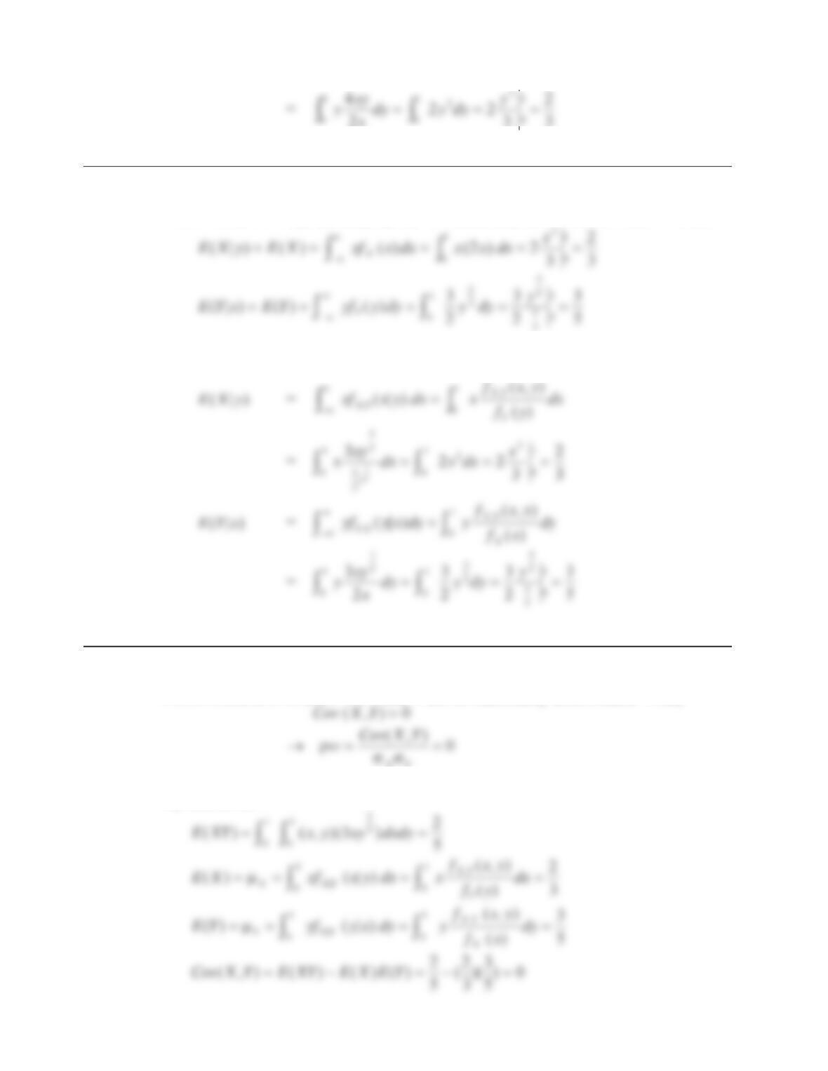
Problem 6-11.
Method 1
From Problem 6-9, fX(x) and fY (y) are for statistically uncorrelated X and Y. Thus,
f
3
3
0
0
Method 2
By definition,
6-6
Problem 6-12.
Model 1
From Problem 6-10, fX (x) and fY (y) are for statistically uncorrelated X and Y. Thus,
Method 2
By definition,
Problem 6-13.
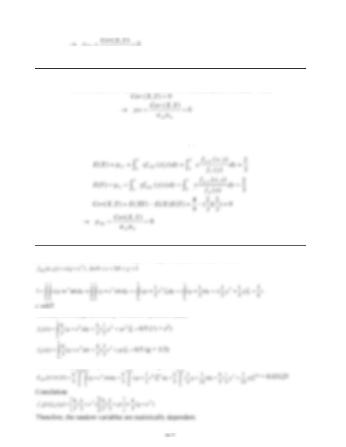
Method 1
From Problems 6-10 and 6-12, X and Y are for statistically uncorrelated. Thus,
XY
Method 2
By definition,
XY
XY
Problem 6-14.
Method 1
From Problems 6-9 and 6-11, X and Y are statistically uncorrelated. Thus,
Method 2
By definition,
EXY xy xydxdy() ()( )
³³
0
1
0
144
9
Problem 6-15.
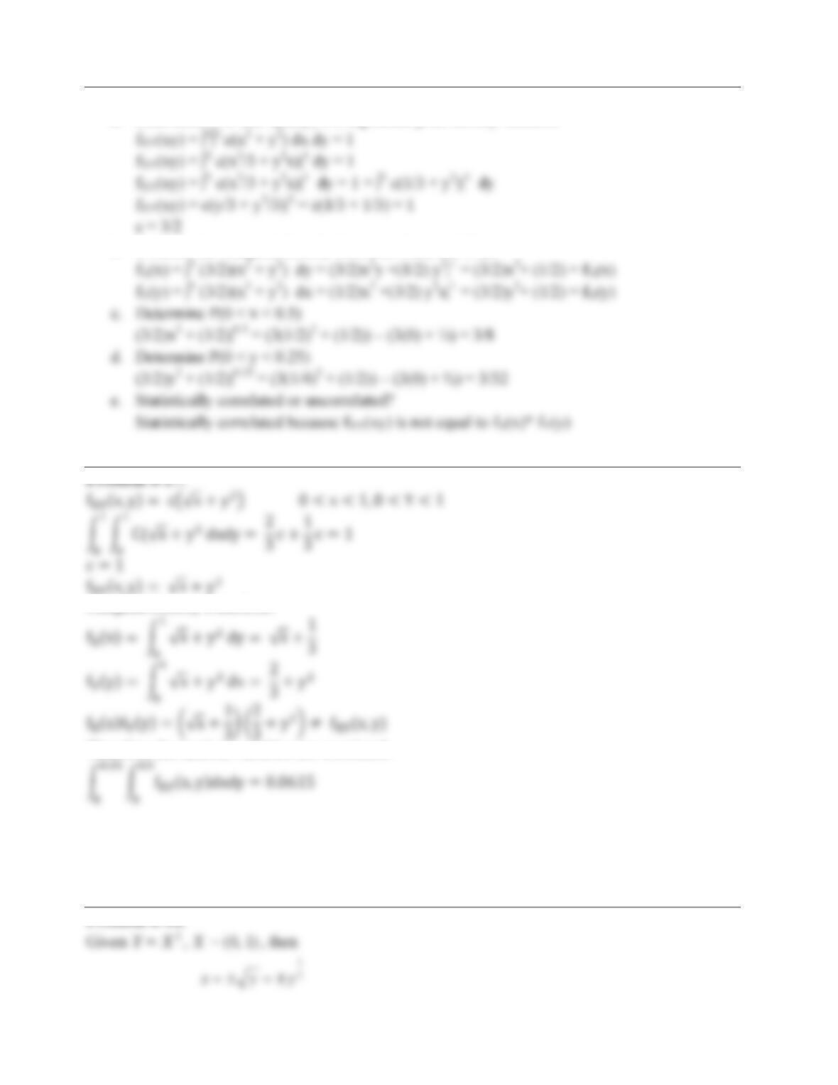
Determine the constant c such that EG
f is a legitimate joint density function.
Evaluate the marginal density functions )(efEand )(gfG.
0
Evaluate the probability that 0<e<0.5 and 0<g<0.25.
6-8
Problem 6-16.
a. Determine c so that fXY(xy) is a legitimate joint density function
b. Evaluate the marginal density functions fX(x) and fY(y)
Marginal Density Functions:
Therefore the random variables are correlated.
6.3. Functions of Random Variables
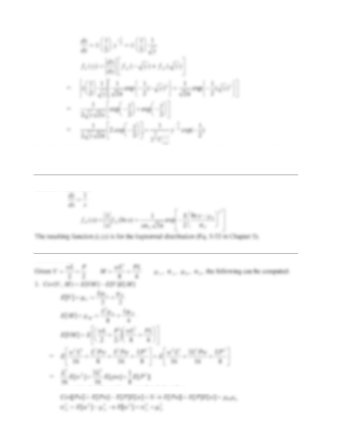
Problem 6-18.
6-9
Therefore, Y follows a chi-square distribution with k=1 in the density function equation of Eq. 5-
55 in Chapter 5.
Problem 6-19.
Given
Y
X
ln , then
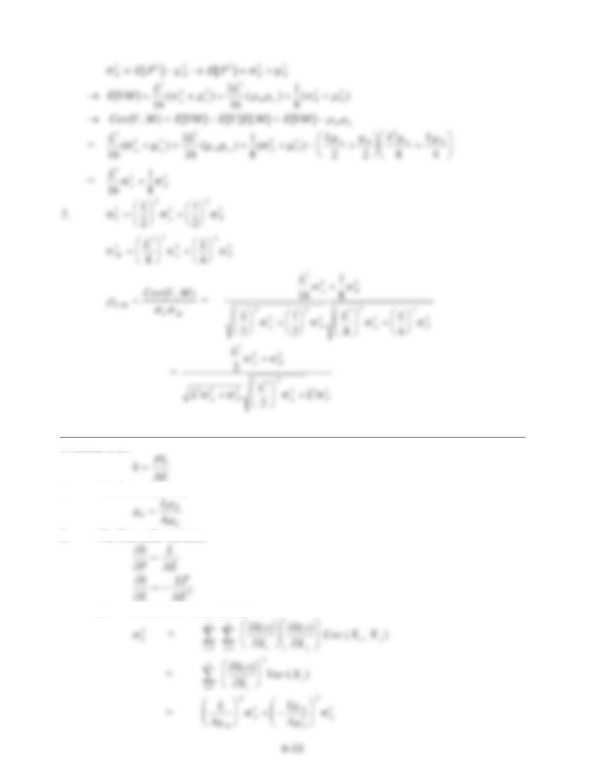
Problem 6-20.
Assuming P and w to be uncorrelated, therefore
Problem 6-21.
1. The first order mean
2. The first order variance
(a) P and E are uncorrelated.
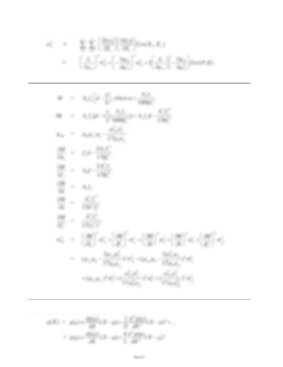
(b) P and Eare correlated.
Problem 6-22.
Problem 6-23.
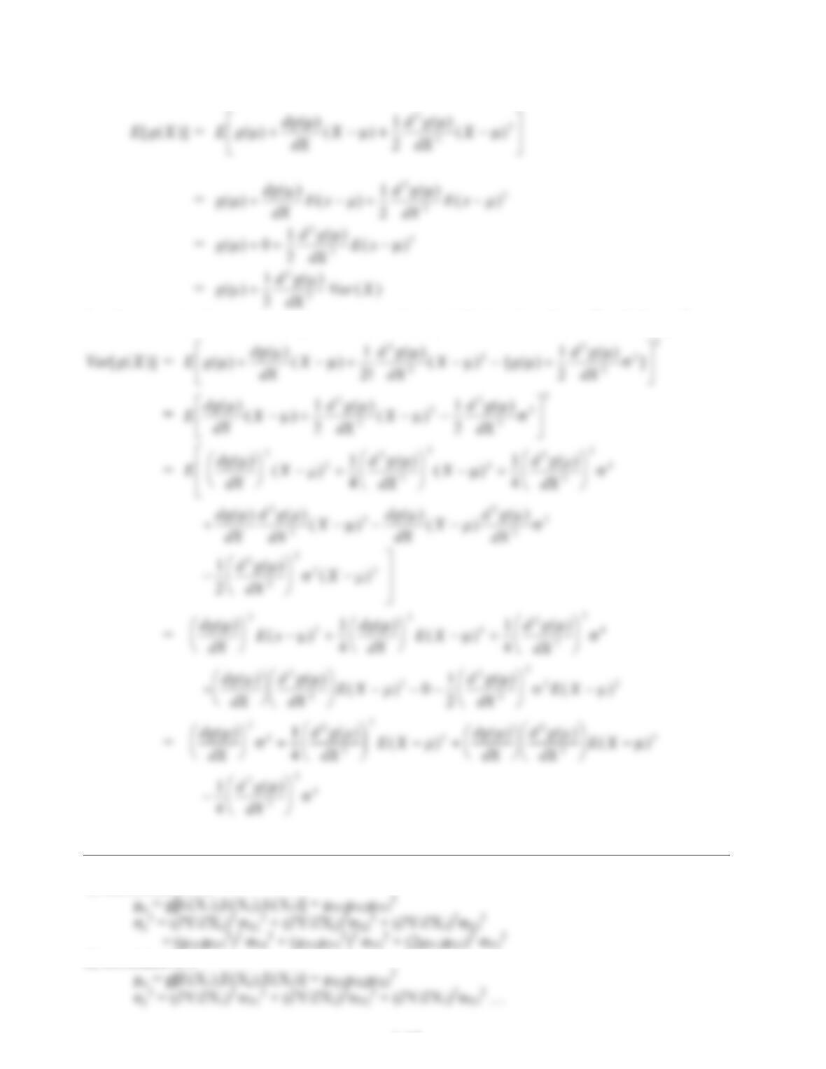
Expand g(X) in Taylor series about the mean value P
6-12
1. The second order mean is given by ( note that by definition P
E
X
()
):
2. The second order variance is given by (note that by definition Var X E X() ( ) VP
22
):
Problem 6-24.
1) uncorrelated X’s
2) correlated X’s
Problem 6-25.
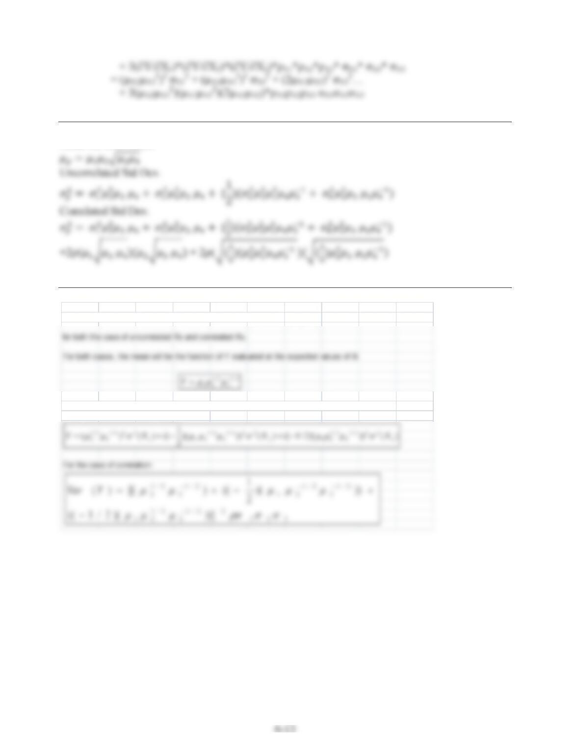
Mean for both cases.
Problem 6-26.
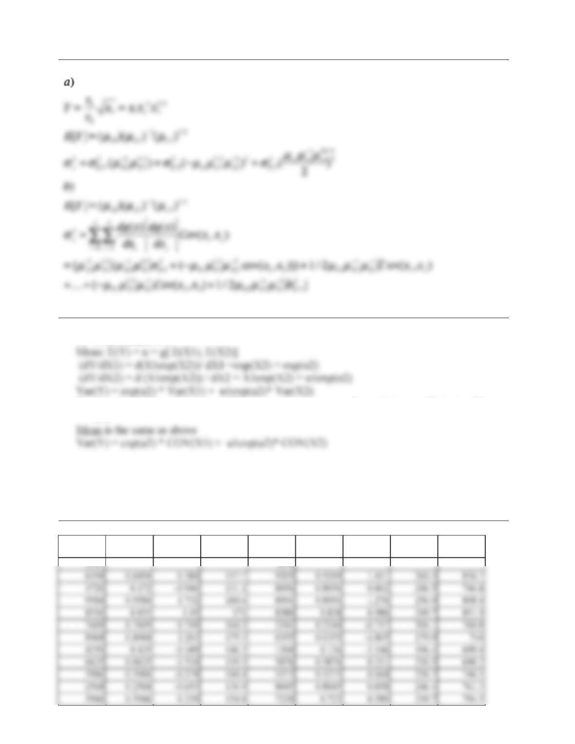
Compute the first order approximate mean and variance for
For the case of uncorrelated X‘s, the variance, Var(Y) will be the sum of the partial derivatives
times the variances of each variable:
2/1
3
2/1
21
XXXY
6-14
Problem 6-27.
Problem 6-28.
1) Uncorrelated X’s
2) Correlated X’s as functions of the mean and variances and correlation coefficients of the
X’s.
6.5. Multivariable Simulation
Problem 6-29.
Random
Number
U1 Z
1 X Random
Number
U2 Z
2 Y C
6-15
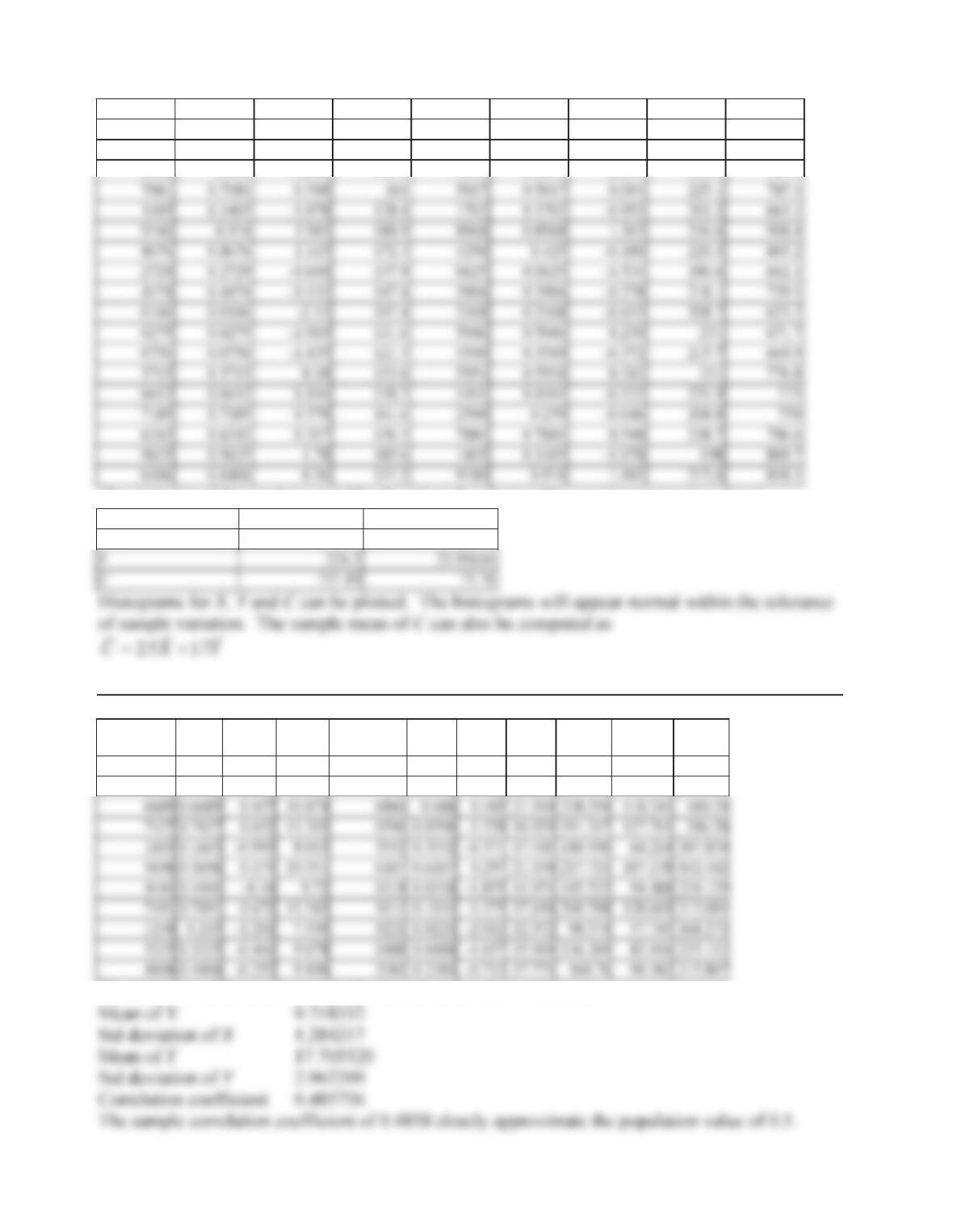
3549 0.3549 -0.372 142.6 1284 0.1284 -1.134 196.7 690.7
5954 0.5954 0.242 154.8 6486 0.6486 0.382 234.5 785.8
4501 0.4501 -0.125 147.5 0681 0.0681 -1.49 187.8 687.9
2590 0.259 –0.646 137.1 4637 0.4637 -0.091 222.7 721.3
The statistics of the random variables based on the above table are (Approximate values)
Random Variable Average Standard Deviation
X150.54 20.97116
Problem 6-30.
Random
Number U1 Z
1 X Random
Number U2 Z
2 Y X*Y X**2 Y**2
9507 2782
383
0
0.383 -0.298 9.405 7395 0.7395 0.642 21.221 199.578 88.449 450.333
0
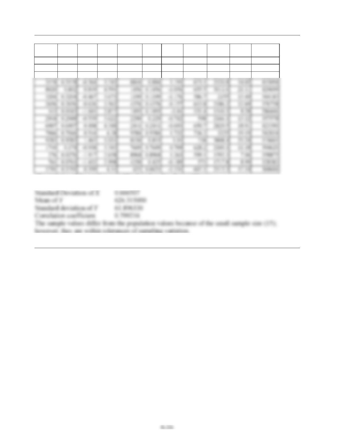
The statistics of the random variables based on the above table are
Problem 6-31.
Random
Number
U1 Z
1 X Random
Number U2 Z
2 Y X*Y X**2 Y**2
1073 6639
1513 0.1513 -1.031 3.278 763 0.0763 -1.431 550.1 1803.6 10.75 302665
2891 0.2891 -0.556 3.611 5821 0.5821 0.207 629.8 2273.9 13.04 396597
The statistics of the random variables based on the above table are
Mean of X 3.723608
Problem 6-32.
Same as problem 6-31 with generated random number using the rand function instead of the mid-
square method.