2-17
6 100-125
7 125-150
8 150-175
9 175-200
10 200-225
Problem 2-25.
Problem 2-26.
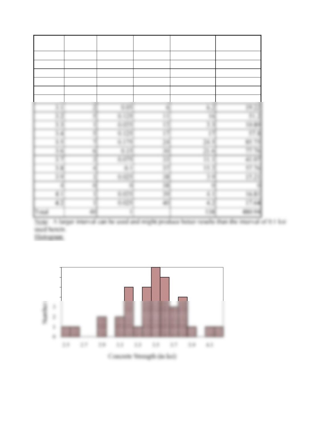
Using an interval of 0.1 ksi, the following table can be constructed.
2-18
Mid-
interval
Count Frequency
(f)
Cumulative
value
x(count) x2(count)
2.5 1 0.025 1 2.5 6.25
2.6 1 0.025 2 2.6 6.76
2.7 0 0 2 0 0
2.8 0 0 2 0 0
2.9 2 0.05 4 5.8 16.82
3 0 0 4 0 0
4
5
6
7
2-19
Frequency Diagram:
0.12
0.14
0.16
0.18
0.2
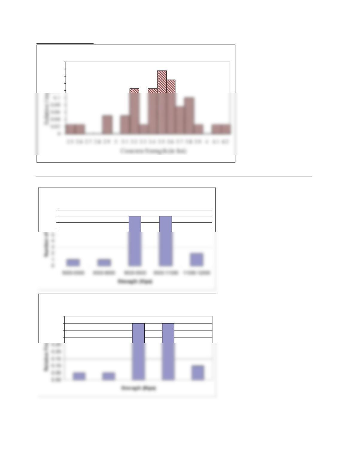
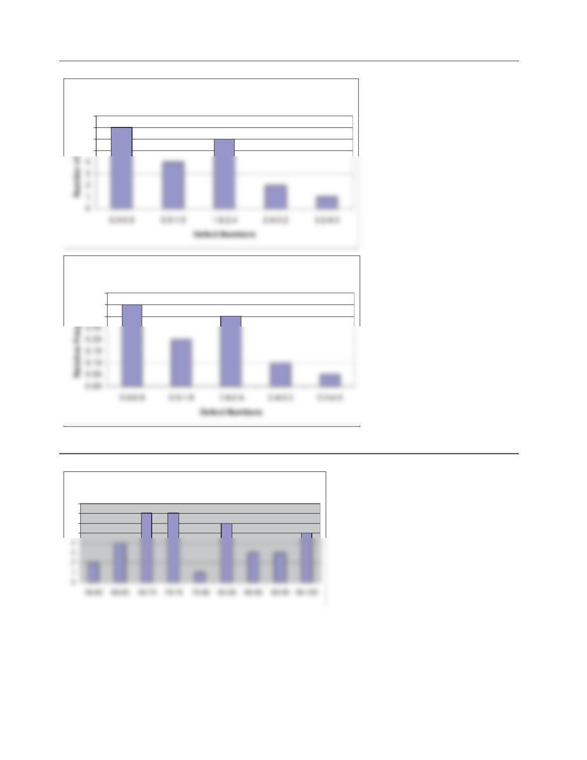
Problem 2-27.
Histogram for pile strength
6
7
8
9
Frequency diagram for pile strength
0.30
0.35
0.40
0.45
2-20
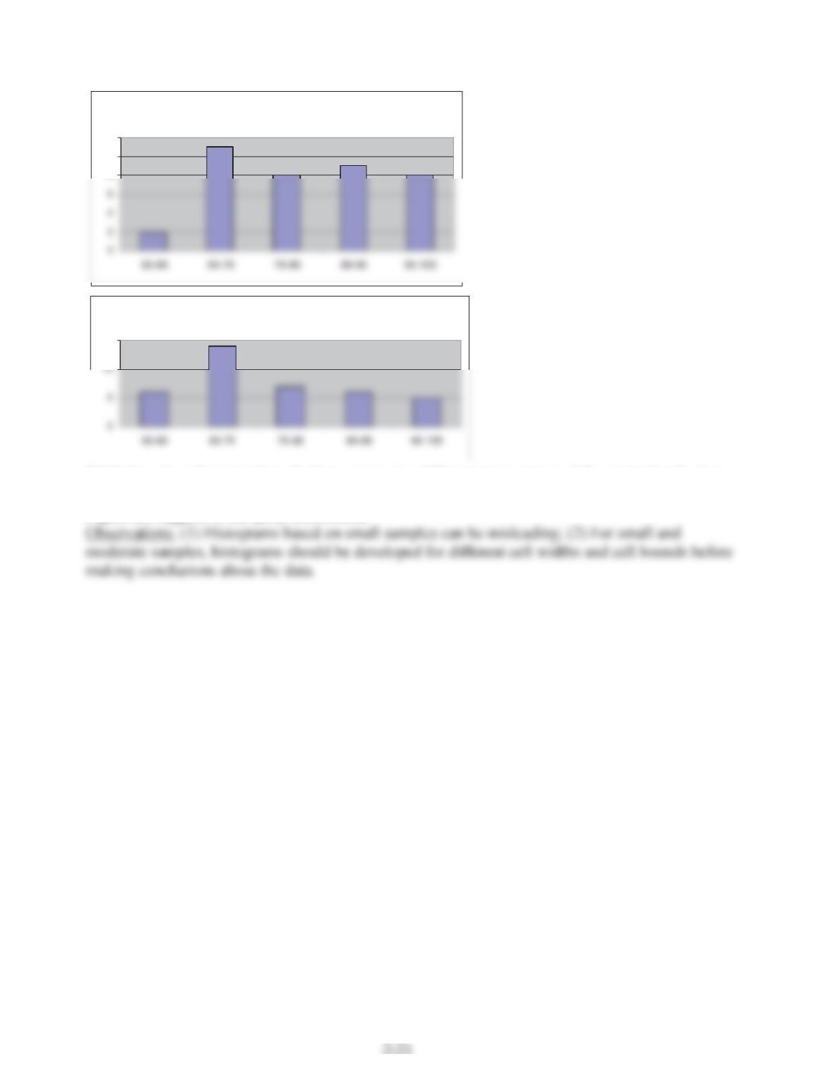
Problem 2-28.
Histogram for number of defects
5
6
7
8
Frequency diagram for number of defects
0.30
0.35
0.40
Problem 2-29.
Case (a)
5
6
7
8
Case (b)
8
10
12
Case (c)
15
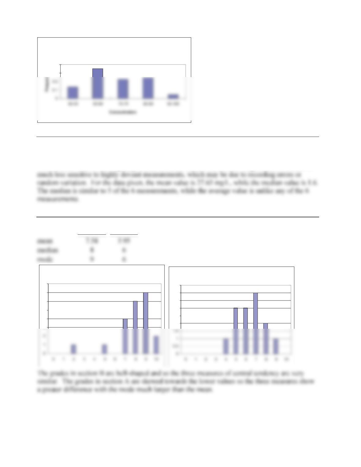
While based on the same data, the histograms give different impressions of the grade distribution.
Figure (a) indicates a two-peaks distribution, while Figure (b) suggests a uniform distribution and
Figure (c) suggests a one-peak distribution.
2-22
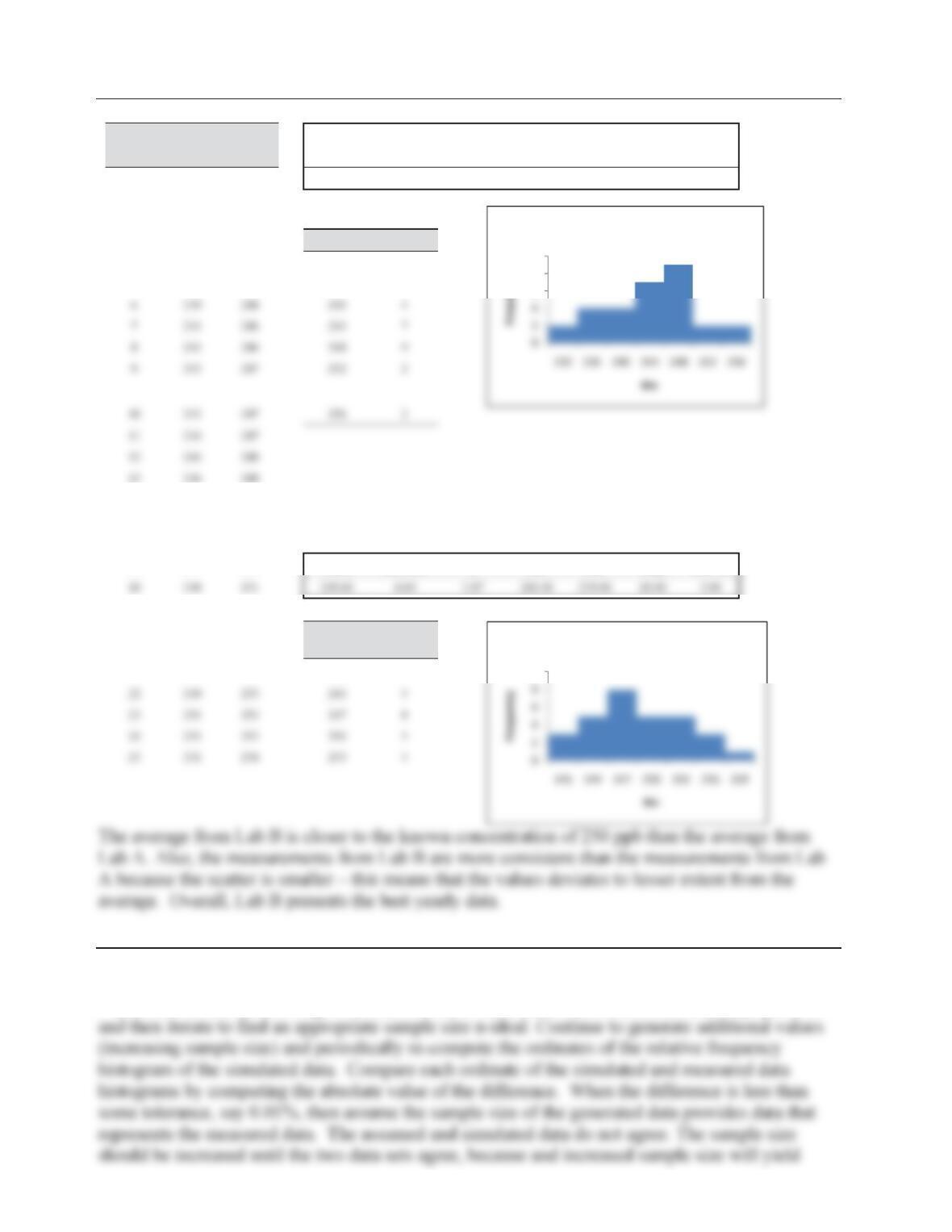
Problem 2-30.
Sample
#LAB A LAB B
Mean Std. Dev. k min max range interval
1 232 241 245.63 6.30 5.87 232.00 256.00 24.00 4.00
2 234 243
3 236 243 Bin Frequency
4 237 244 232 2
5 237 244 236 4
14 246 249
15 246 249
16 247 249
17 247 251 Mean Std. Dev. k min max range interval
19 248 251
20 248 252 Bin Frequency
21 249 252 241 3
6
8
10
LABA
10
LABB
Problem 2-31.
Using the random number generation feature of excel, you could estimate various sample sizes (n
= 25,50,100, ect.) to find rough boundaries which overestimate and underestimate the population
2-23
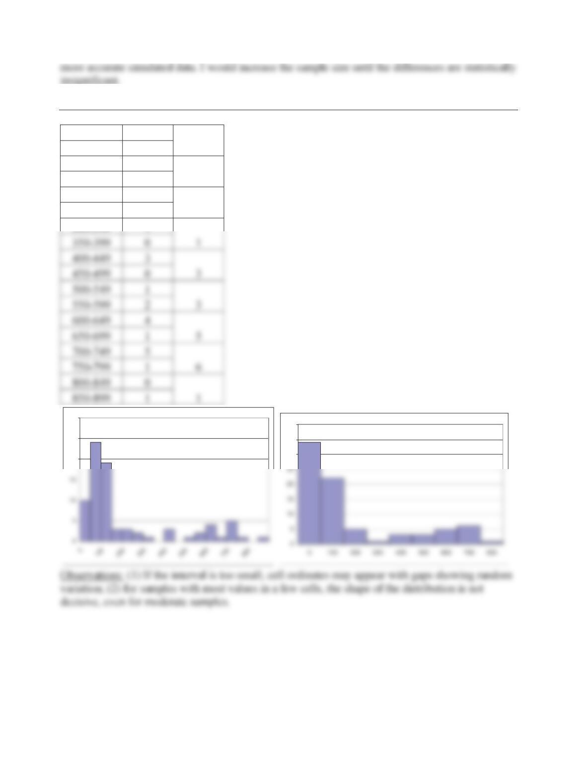
Problem 2-32.
0-49 10
34
50-99 24
100-149 19
22
150-199 3
200-249 3
5
250-299 2
300-349 1
20
25
30
30
35
40
2-24
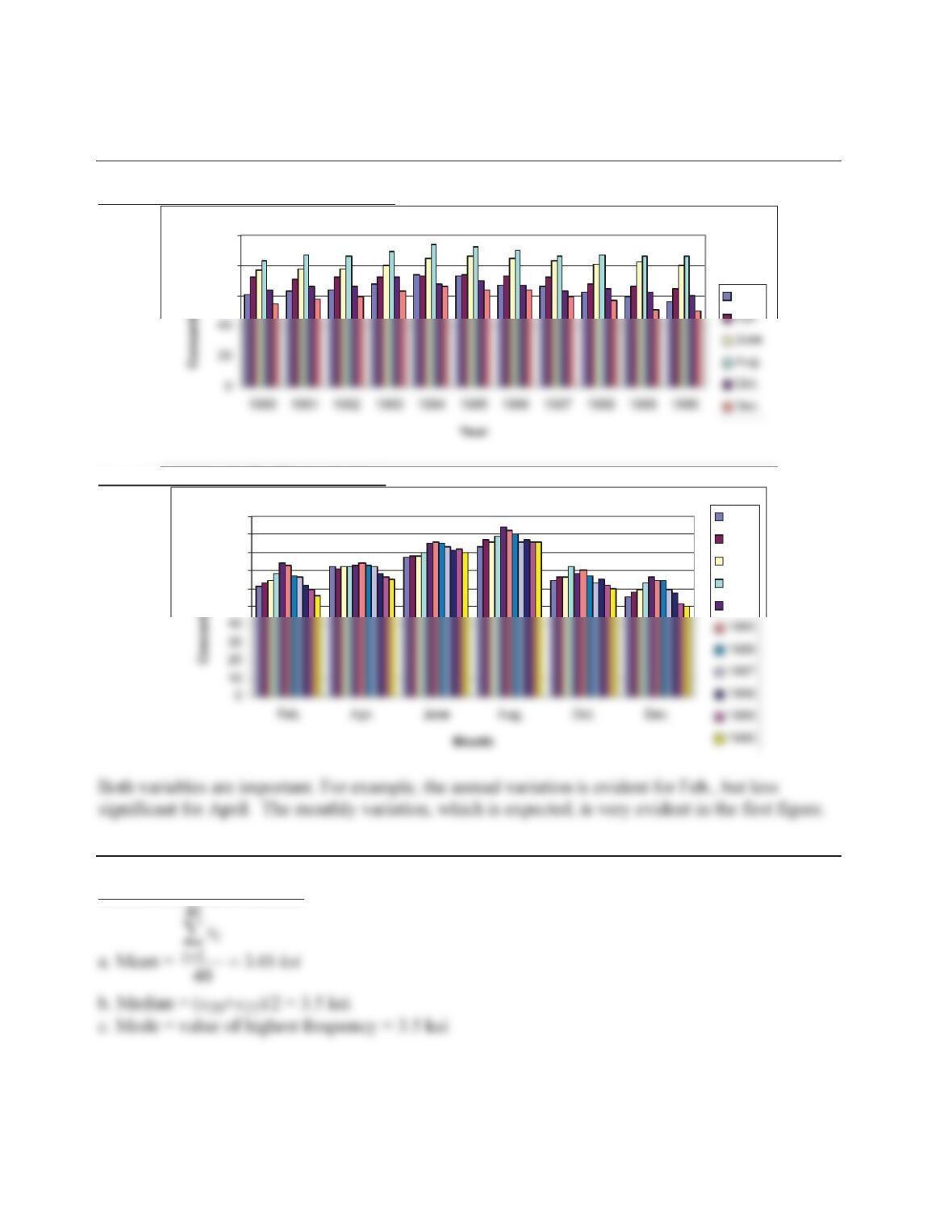
2.6. Descriptive Measures
Problem 2-33.
Monthly variation in the Concentration:
60
80
100
Feb.
Annual variation in the Concentration:
50
60
70
80
90
100
1980
1981
1982
1983
1984
Problem 2-34.
Central tendency measures:
2-25
Problem 2-35.
Central tendency measures:
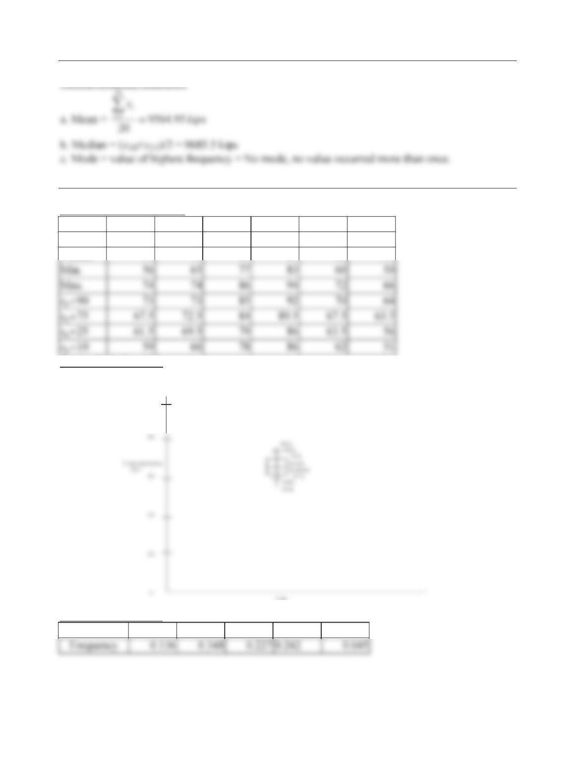
Problem 2-36.
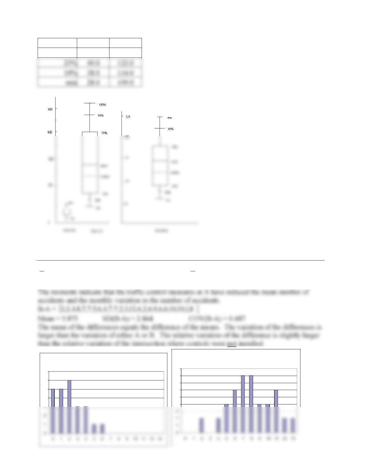
Box-and-whisker plot data:
Feb. Apr. June Aug. Oct. Dec.
Mean 64.82 70.73 81.36 87.82 65.73 58.73
Median 64 72 81 87 66 59
Box-and-whisker plot:
The following is the box-and-whisker plot constructed only for the month of February. For
multiple box and whisker plots display, refer to Section 2.5.4 and Figure 2-16 of the textbook.
100
Feb.
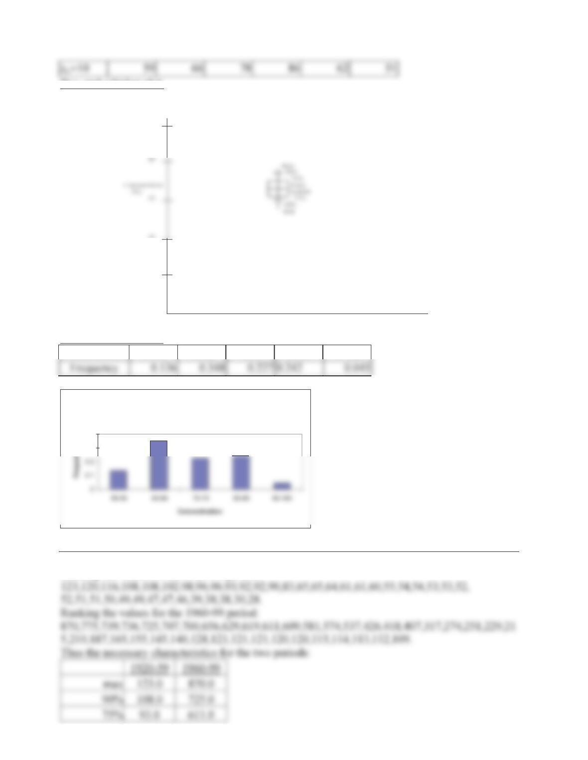
Frequency Histogram:
Concentration 50-59 60-69 70-79 80-89 90-100
2-26
Frequency Histogram of Maximum Daily Ozone
Concentration
0.3
0.4
Problem 2-37.
Mean = sum/6 = 165.9/6 = 27.65 mg/l
Median = 1.6 mg/l
The extreme value of 157.9 greatly affects the mean but not the median. In general, the median is
Problem 2-38.
Section A Section B
Section A
3
4
5
6
7
8
Section B
2
2.5
3
3.5
4
4.5
2-27
Problem 2-39.
¦
k
iii xfX 1 where k is the integer number of scores of xi and fiis the frequency of the
Problem 2-40.
Problem 2-41.
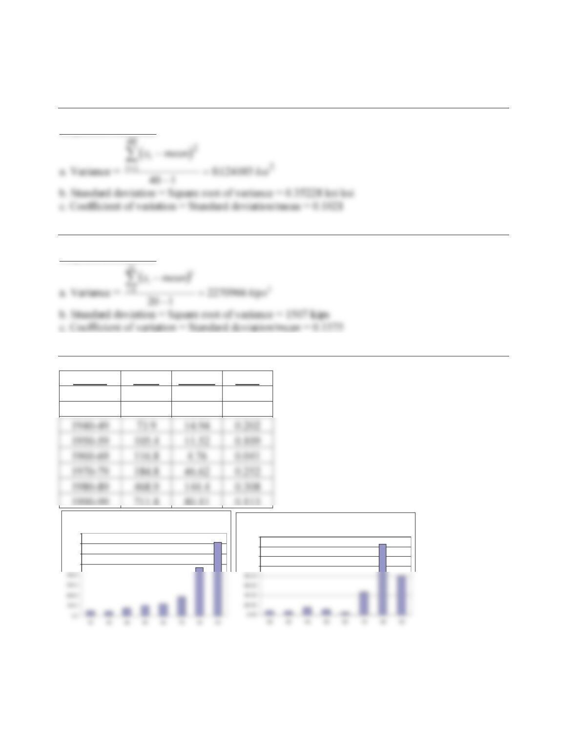
Decade Mean St. Dev. COV
1920-29 48.5 8.21 0.169
1930-39 45.1 7.78 0.173
1940-49 73.9 14.94 0.202
Mean
500.0
600.0
700.0
800.0
Standard Deviation
100.00
120.00
140.00
160.00
COV
0.3
0.35
2-28
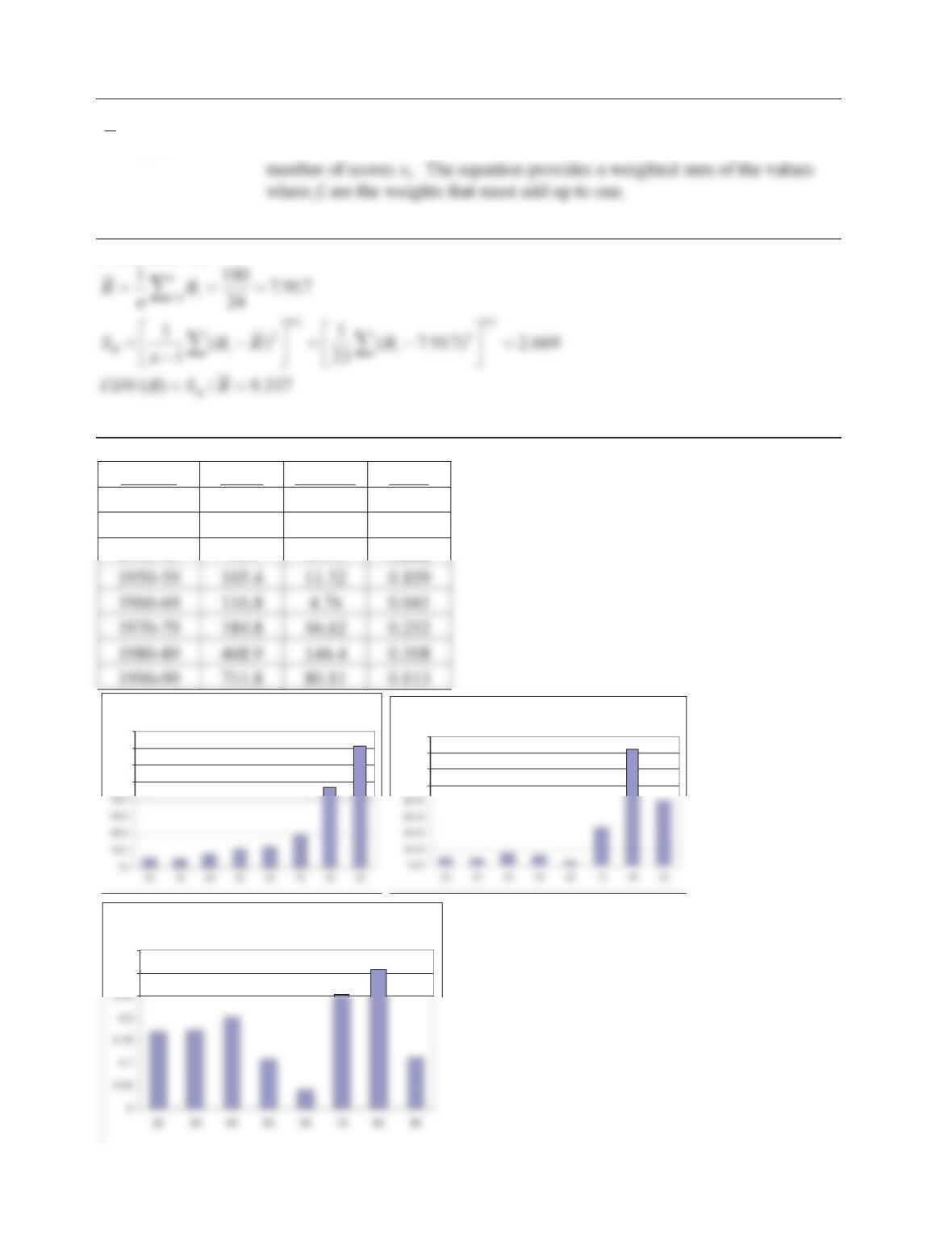
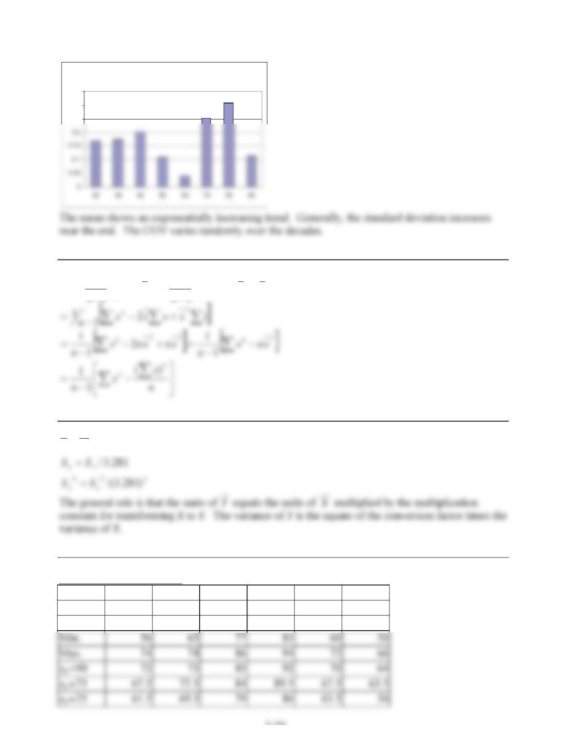
The mean shows an exponentially increasing trend. Generally, the standard deviation increases
near the end. The COV varies randomly over the decades.
Problem 2-42.
Dispersion measures:
Problem 2-43.
Dispersion measures:
Problem 2-44.
Decade Mean St. Dev. COV
1920-29 48.5 8.21 0.169
1930-39 45.1 7.78 0.173
1990-99 711.8 80.11 0.113
Mean
500.0
600.0
700.0
800.0
Standard Deviation
100.00
120.00
140.00
160.00
2-29
COV
0.25
0.3
0.35
Problem 2-45.
¦¦
xxxx
xx
S
2
222
)2(
1
)(
1
Problem 2-46.
281.3/
XY
Problem 2-47.
Box-and-whisker plot data:
Feb. Apr. June Aug. Oct. Dec.
Mean 64.82 70.73 81.36 87.82 65.73 58.73
Median 64 72 81 87 66 59
2-30
Box-and-whisker plot:
The following is the box-and-whisker plot constructed only for the month of February. For
multiple box and whisker plots display, refer to Section 2.5.4 and Figure 2-16 of the textbook.
100
40
20
0
Feb.
Frequency Histogram:
Concentration 50-59 60-69 70-79 80-89 90-100
Frequency Histogram of Maximum Daily Ozone
Concentration
0.3
0.4
Problem 2-48.
Ranking the values for the 1920-59 period:
2-31
mean 68.2 370.6
median 57.5 262.5
Problem 2-49.
042.2 A Standard deviation, SD (A) = 1.681 917.7 B SD(B) = 2.669
COV(A) =0.823 COV(B) =0.337
Intersection A
4
5
6
7
Intersection B
2
3
3
4
4
5