Chapter 19: Probability and Statistics in Engineering
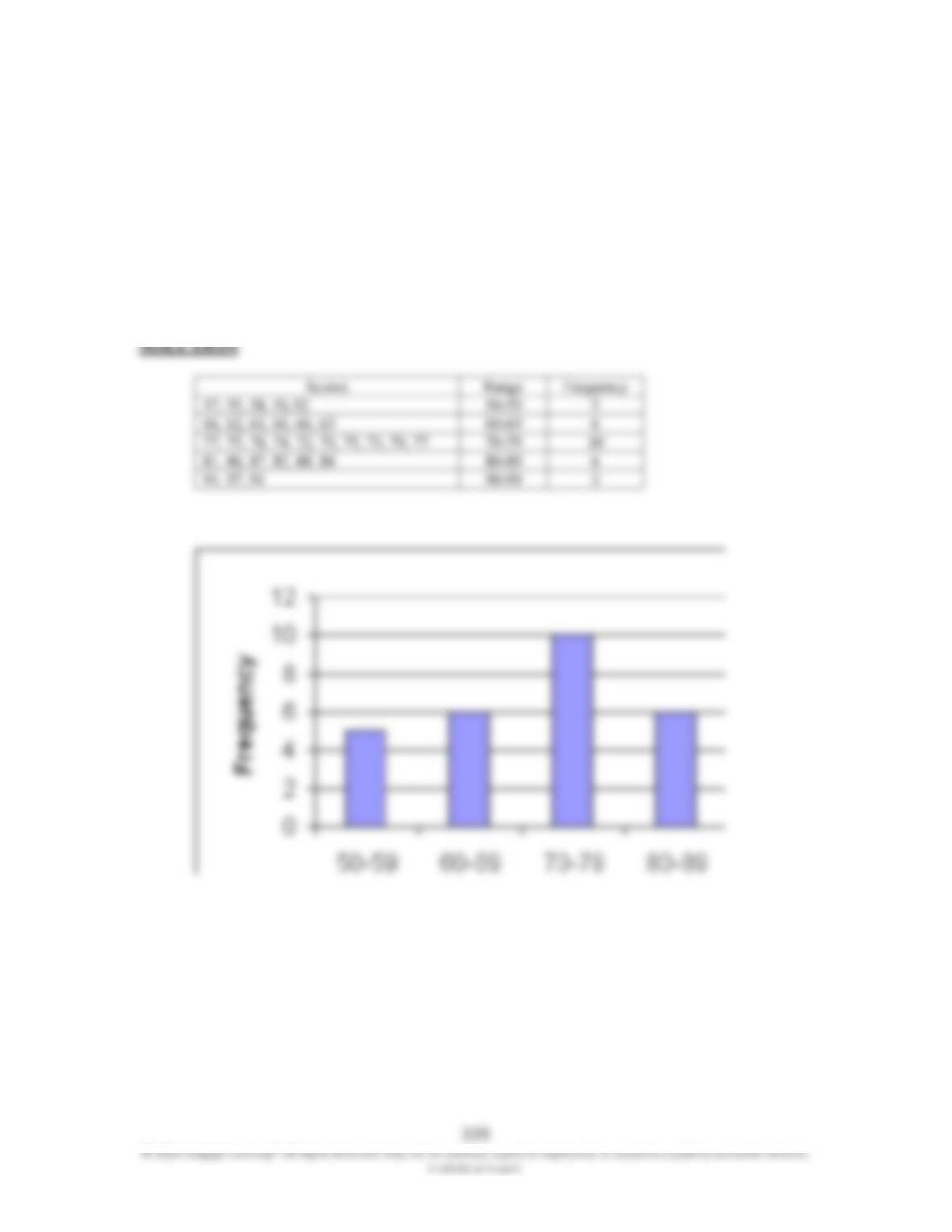
19.1 The scores of a test for an engineering class of 30 students are shown here.
Organize the data in a manner similar to Table 19.1 and use Excel to create a
histogram.
Scores: 57, 94, 81, 77, 66, 97, 62, 86, 75, 87, 91, 78, 61, 82, 74, 72, 70,
88, 66, 75, 55, 66, 58, 73, 79, 51, 63,77, 52, 84
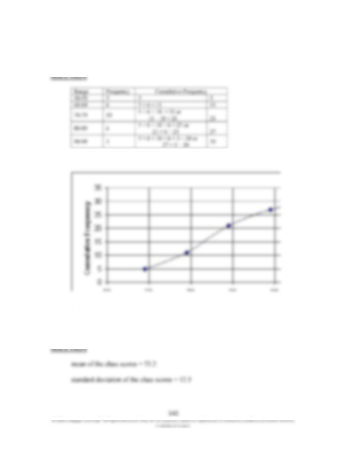
19.2 For Problem 19.1 calculate the cumulative frequency and plot a cumulative
frequency polygon.
Cumulative
–
5
5
5
–
6
5 + 6 = 11
11 + 10 = 21
21 + 6 = 23
27 + 3 = 30
19.3 For Problem 19.1, using Equations (19.1) and (19.6), calculate the mean and
standard deviation of the class scores.
341
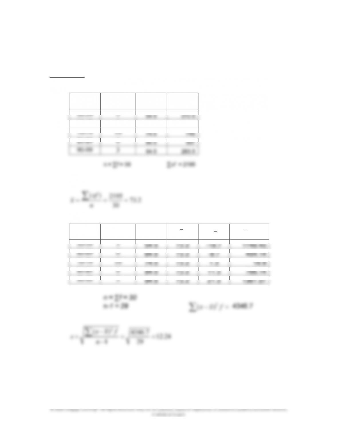
19.4 For Problem 19.1, using Equations (19.7) and (19.8), calculate the mean and
standard deviation of the class scores.
SOLUTION
Range
Frequency
f
midpoint
x
xf
60-69 6 64.5 387
30
n
Range Frequency
f
midpoint
x
54.5
73.2
–
18.7
64.5
73.2
–
8.7
454.14
74.5
73.2
1.3
1
6
.
9
84.5
73.2
11.3
766.14
94.5
73.2
21.3
n =
∑f = 30
n
–
1 = 29
4
346.7
x
x
fxx 2
)(
x

19.5 For Problem 19.1, calculate the probability distribution and plot the probability-
distribution curve.
SOLUTION
Range
Frequency
Probability
5 0.167
∑p = 1
19.6 In order to improve the production time, the supervisor of assembly lines in a
manufacturing setting of cellular phones has studied the time that it takes to
assemble certain parts of a phone at various stations. She measures the time that it
takes to assemble a specific part by 165 people at different shifts and on different
days. The record of her study is organized and shown in the accompanying table.
Time that it takes a person to
assemble the part (minutes)
Frequency
4
15
5
20
6
28
7
34
8
28
9
24
10
16
Plot the data and calculate the mean and standard deviation.
SOLUTION
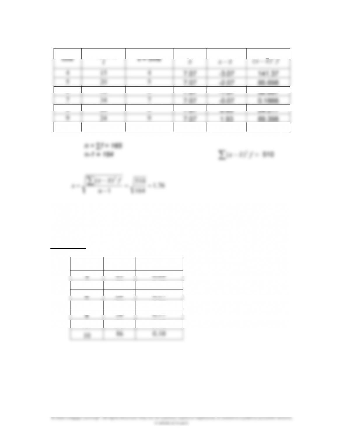
7.07
–
3.07
141.37
7.07
–
2.07
85.698
7.07
–
1.07
32.057
7.07
–
0.07
0.1666
7.07
0.93
24.217
7.07
1.93
89.398
10 16 10
7.07
2.93
137.36
n =
∑f = 165
fxx 2
)(
n
–
1
=
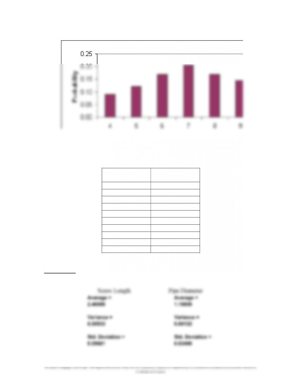
19.8 Determine the average, variance, and standard deviation for the following parts.
The measured values are given in the accompanying table.
Screw Length
(cm)
Pipe Diameter
(in.)
2.55
1.25
2.45
1.18
2.55
1.22
2.35
1.15
2.60
1.17
2.40
1.19
2.30
1.22
2.40
1.18
2.50
1.17
2.50
1.25
SOLUTION
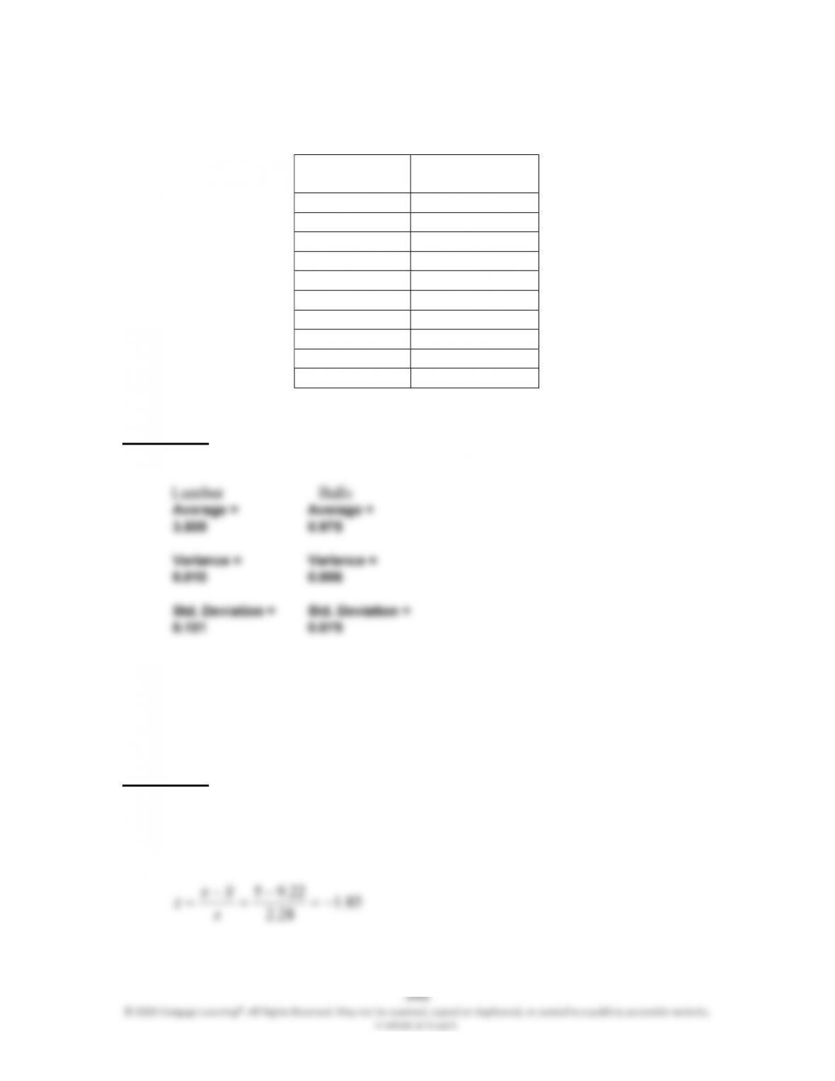
19.9 Determine the average, variance, and standard deviation for the following parts.
The measured values are given in the accompanying table.
2 x 4 Lumber
Width (in.)
Steel Spherical
Balls (cm)
3.50
1.00
3.55
0.95
3.45
1.05
3.60
1.10
3.55
1.00
3.40
0.90
3.40
0.85
3.65
1.05
3.35
0.95
3.60
0.90
SOLUTION
19.13 For Example 19.4, determine the probability that it will take a person between 5
and 10 minutes to assemble the computer parts.
SOLUTION
The value 5 is below the mean value and the z value corresponding to 5 is
determined from
28
.
2
s
347
© 2020 Cengage Learning®. All Rights Reserved. May not be scanned, copied or duplicated, or posted to a publicly accessible website,
in whole or in part.
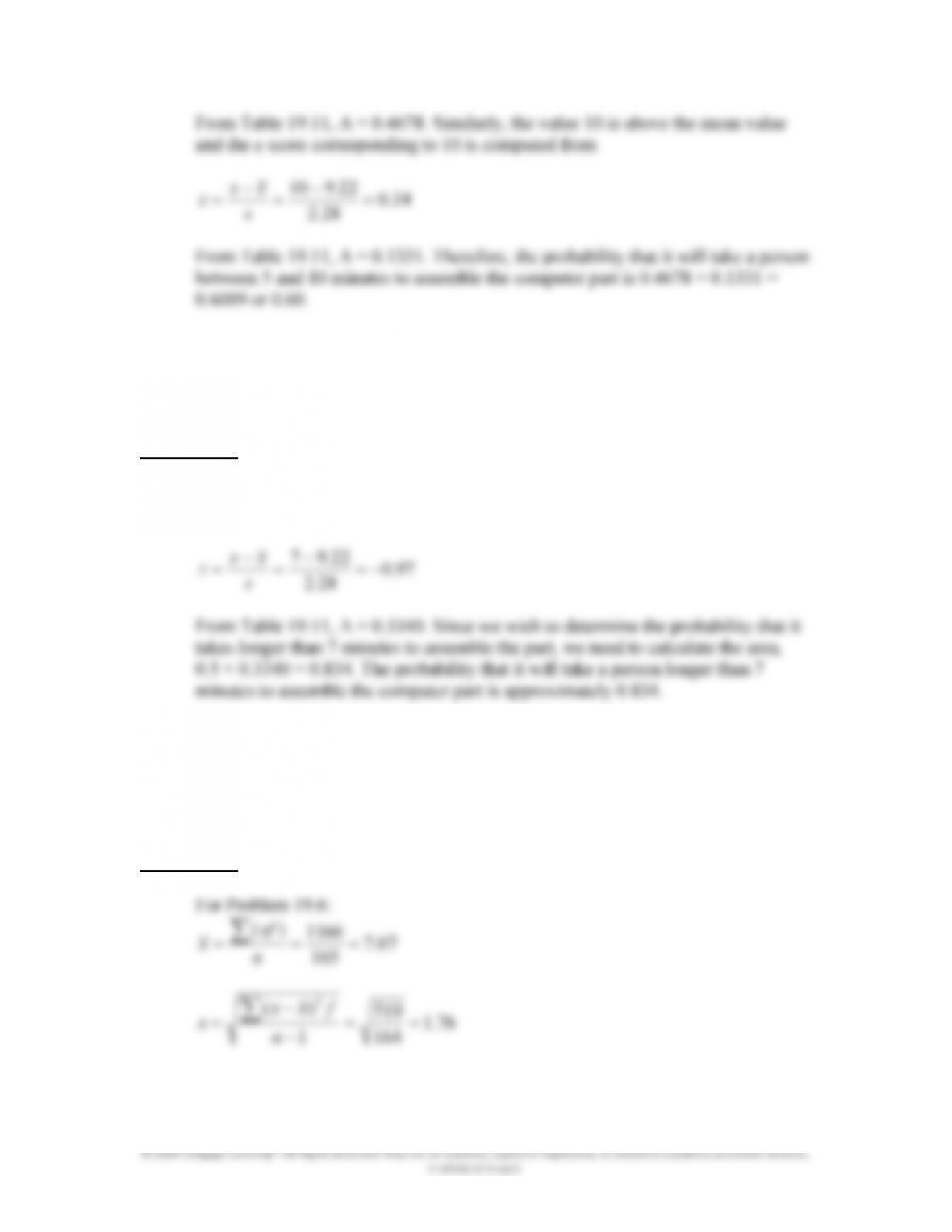
From Table 19.11, A = 0.4678. Similarly, the value 10 is above the mean value
and the z score corresponding to 10 is computed from
34.0
28
.
2
22.910
s
xx
z
From Table 19.11, A = 0.1331. Therefore, the probability that it will take a person
between 5 and 10 minutes to assemble the computer part is 0.4678 + 0.1331 =
0.6009 or 0.60.
19.14 For Example 19.4, determine the probability that it will take a person longer than
7 minutes to assemble the computer parts.
SOLUTION
For this problem, the z score is
19.15 For Problem 19.6, (assuming normal distribution), determine the probability that
it will take a person between 5 to 8 minutes to assemble the phone.
SOLUTION
164
1
n
28
.
2
s
348
The value 5 is below the mean value and the z value corresponding to 5 is
determined from
19.16 Imagine that you and four of your classmates have measured the density of air and
recorded the values shown in the accompanying table. Determine the average,
variance, and standard deviation for the measured density of air.
Density of
Air (kg/m3)
1.27
1.21
1.28
1.25
1.24
SOLUTION
Density of
Air
deviation
19.17 Imagine that you and four of your classmates have measured the viscosity of
engine oil and recorded the values shown in the accompanying figure. Determine
the average, variance, and standard deviation for the measured viscosity of oil.
Viscosity of
Engine Oil
(N.s/m2)
0.15
0.10
0.12
0.11
0.14
SOLUTION
Viscosity of
Engine Oil
Average
19.18 Assuming a standard normal distribution (Table 19.11), what percentage of the
data falls between −1.5 s to 1.5 s?
350
19.19 Assuming a standard normal distribution (Table 19.11), what percentage of the
data falls between − 0.5 s to 0.5 s?
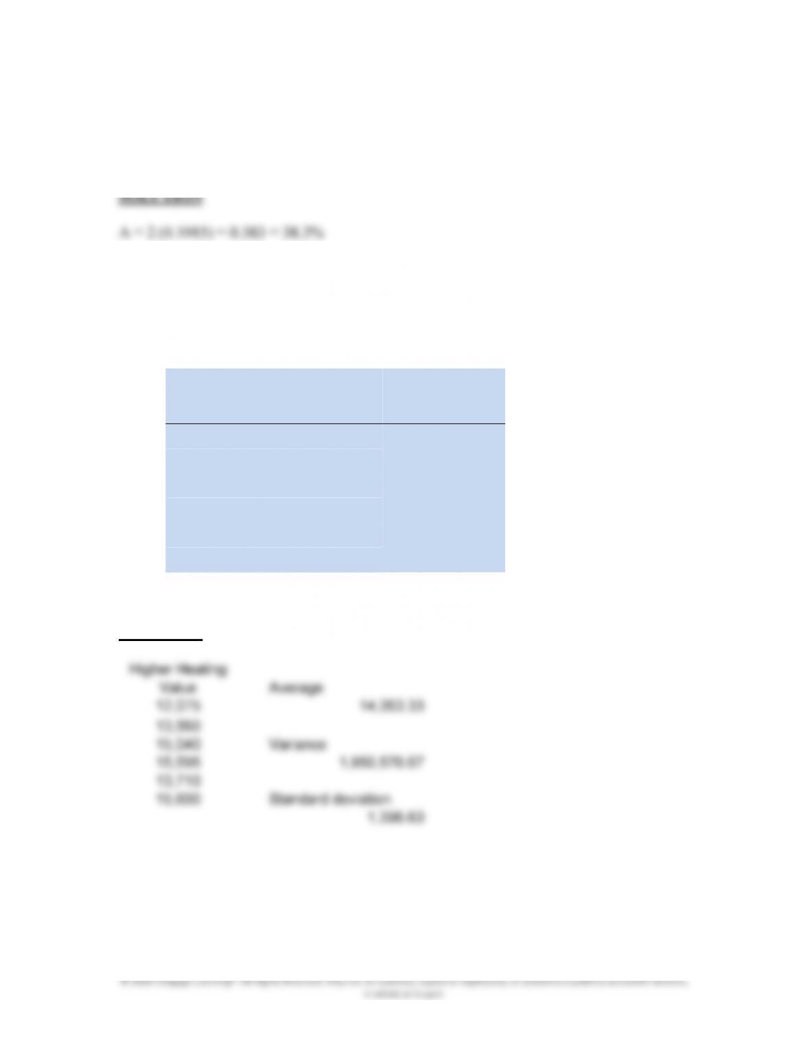
19.20 Typical heating values of coal from various part of U.S. are shown in the
accompanying table. Calculate the average, variance, and standard deviation for
the given data.
Coal from County
and State of
Higher Heating
Value
(Btu/lbm)
Musselshell, Montana 12,075
Emroy, Utah 13,560
Pike, Kentucky 15,040
Cambria, Pennsylvania 15,595
Williamson, Illinois 13,710
McDowell, West Virginia 15,600
Source: Babcock and Wilcox Company, Stream: Its Generation and Use.
SOLUTION
14,263.33
1,950,576.67
1,396.63
351
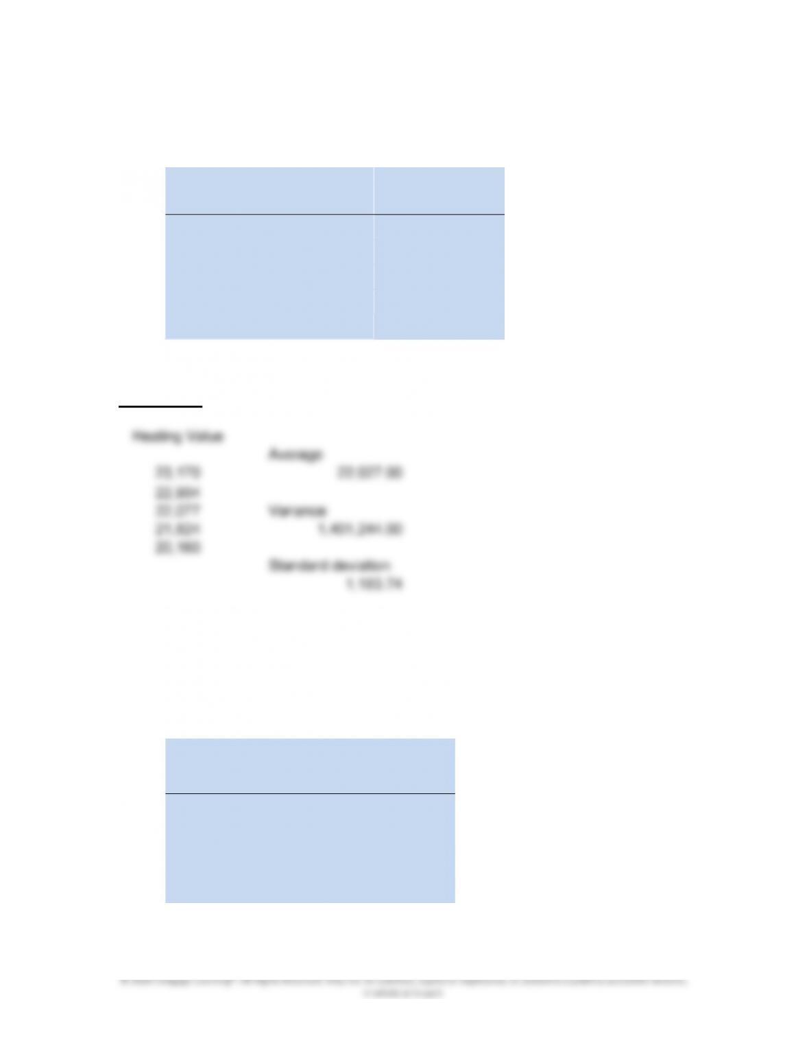
19.21 Typical heating values of natural gas from various part of the U.S. are shown in
the accompanying table. Calculate the average, variance, and standard deviation
for the given data.
Source of Gas
Heating Value
(Btu/lbm)
Pennsylvania 23,170
Southern California 22,904
Ohio 22,077
Louisiana 21,824
Oklahoma 20,160
Source: Babcock and Wilcox Company, Stream: Its Generation and Use.
SOLUTION
22,027.00
1,401,244.00
1,183.74
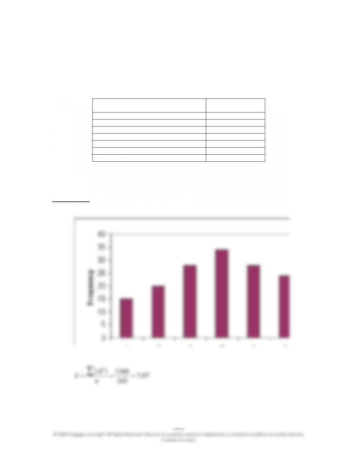
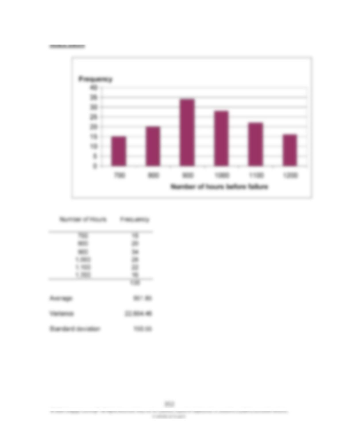
19.22 As an electrical engineer, you have designed a new efficient light bul. In order to
predict its life expectancy, you conducted a series of experiments on 135 of these
light bulbs and gathered the following data. Plot the data and calculate the mean
and standard deviation.
Number of Hours the
Light Bulb Functioned
before Failing Frequency
700
15
800
20
900
34
1000
28
1100
22
1200
16
352
© 2020 Cengage Learning®. All Rights Reserved. May not be scanned, copied or duplicated, or posted to a publicly accessible website,
in whole or in part.
SOLUTION
Number of Hours Frequency
700 15
800 20
900 34
1,000 28
1,100 22
1,200 16
135
Average
951.85
Variance
22,664.46
Standard deviation
150.55
0
5
10
15
20
25
30
35
40
700 800 900
1000
1100 1200
Number of hours before failure
Frequency