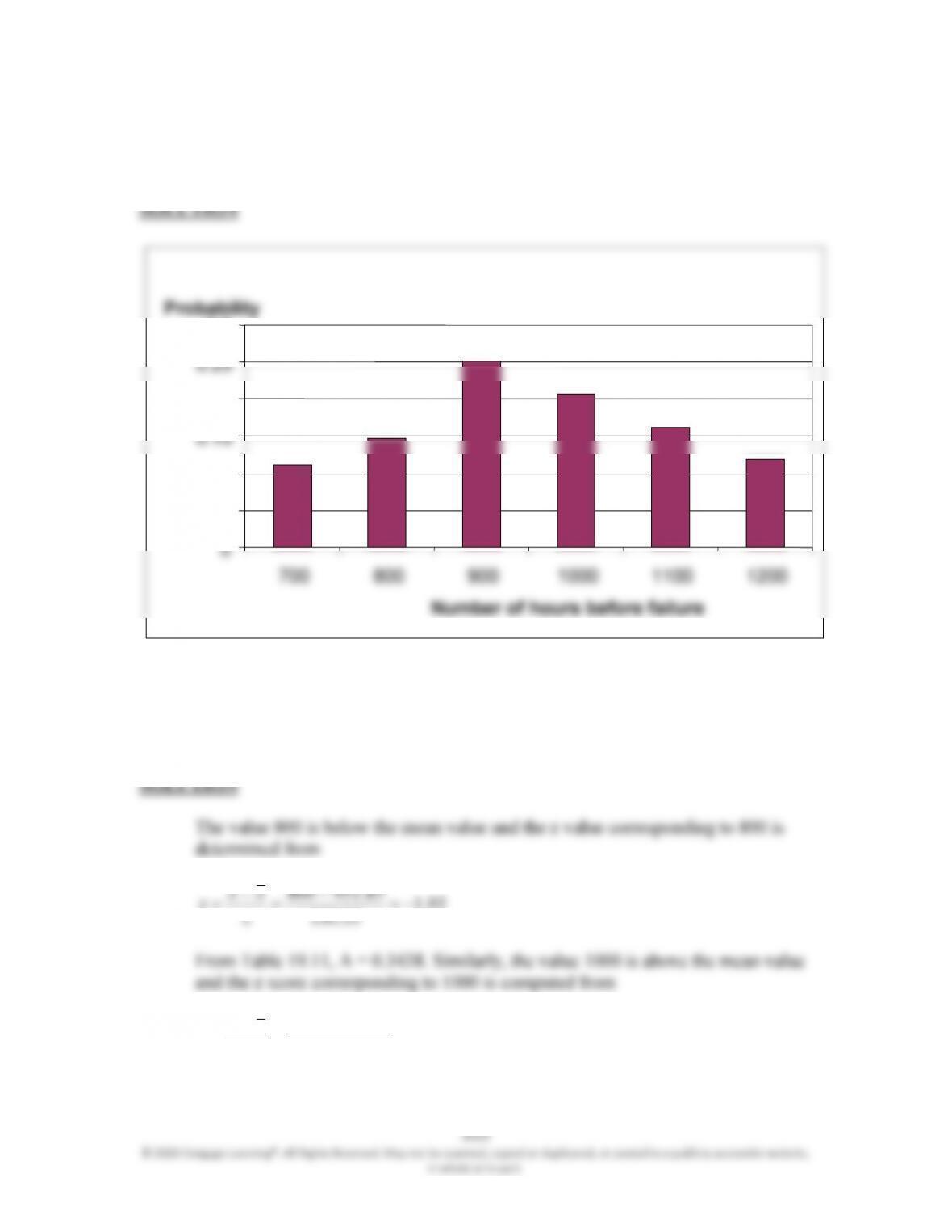
19.23 For Problem 19.22, calculate the probability distribution and plot the probability
distribution curve.
19.24 For Problem 19.22, determine the probability (assuming normal distribution) that
a light bulb would have a life expectancy between 800 and 1000 hours.
01.1
55
.
150
s
z
32.0
54
.
150
85.9511000
s
xx
z
0.05
0.1
0.15
0.2
0.25
0.3
Number of hours before failure
Probability
354
© 2020 Cengage Learning®. All Rights Reserved. May not be scanned, copied or duplicated, or posted to a publicly accessible website,
in whole or in part.
From Table 19.11, A = 0.1255. Therefore, the probability that a light bulb would
have a life expectancy between 800 and 1000 hours is 0.3438+0.1255 = 0.4693
19.25 For Problem 19.22 determine the probability (assuming normal distribution) that a
light bulb would have a life expectancy greater than 1000 hours.
32.0
54
.
150
s
z
19.26 For Problem 19.22, determine the probability (assuming normal distribution) that
a light bulb would have a life expectancy less than 900 hours.
34.0
54
.
150
85.951900
s
xx
z
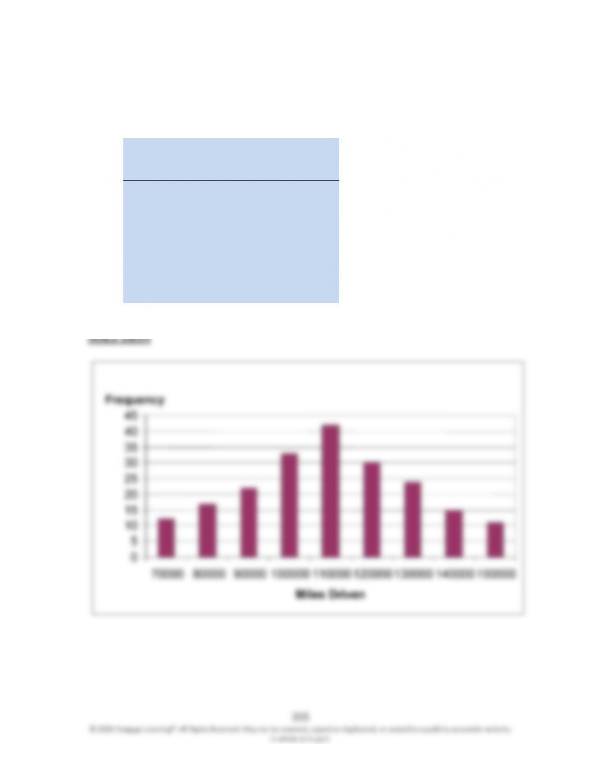
19.27 As a mechanical engineer working for an automobile manufacturer, you conduct a
survey and collect the following data in order to study the performance of an
engine that was designed many years ago. Plot the data and calculate the mean
and standard deviation.
Miles Driven before
a Need for An
Engine Maintenance Frequency
70,000
12
80,000
17
90,000
22
100,000
33
110,000
4
2
120,000
30
130,000
24
140,000
15
150,000
11
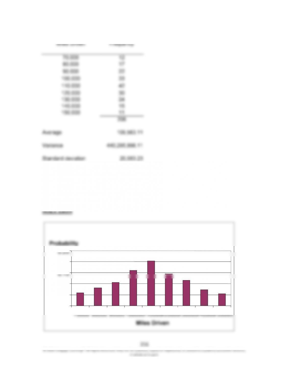
20,983.23
19.28 For Problem 19.27, calculate the probability distribution and plot the probability
distribution curve.
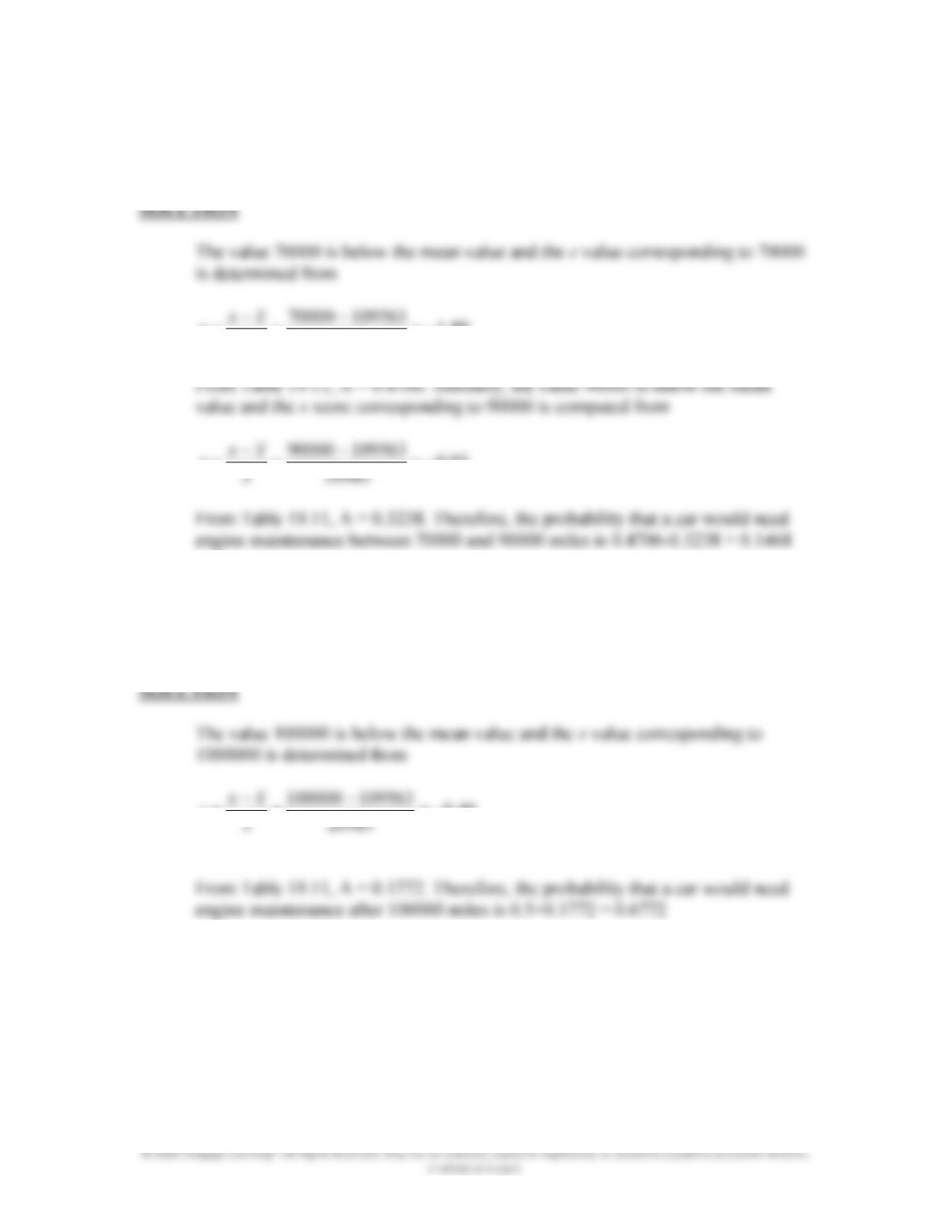
19.29 For Problem 19.27, determine the probability (assuming normal distribution) that
a car would need engine maintenance between 70,000 and 90,000 miles.
358
© 2020 Cengage Learning®. All Rights Reserved. May not be scanned, copied or duplicated, or posted to a publicly accessible website,
in whole or in part.
SOLUTION
The value 85,000 is below the mean value and the z value corresponding to 85000
is determined from
17.1
20983
10956385000
s
xx
z
19.32 For Problem 19.27, determine the probability (assuming normal distribution) that
a car would need engine maintenance before 90,000 miles.
93.0
20983
10956390000
s
xx
z
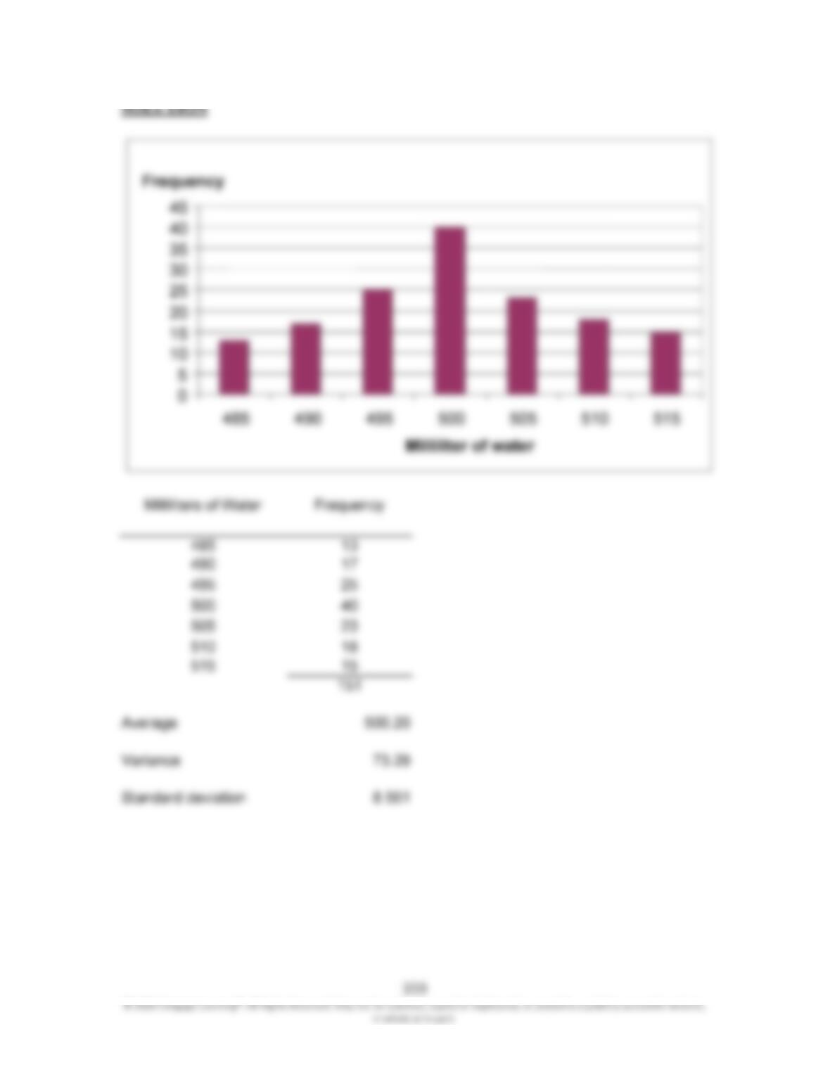
19.33 As an engineer working for a water bottling company, you collect the following
data in order to test the performance of the bottling systems. Plot the data and
calculate the mean and standard deviation.
Milliliters of Water
in the Bottle Frequency
485
13
490
17
495
25
500
40
505
23
510
18
515
15
359
© 2020 Cengage Learning®. All Rights Reserved. May not be scanned, copied or duplicated, or posted to a publicly accessible website,
in whole or in part.
SOLUTION
Milliliters of Water Frequency
485 13
490 17
495 25
500 40
505 23
510 18
515 15
151
Average
500.20
Variance
73.29
Standard deviation 8.561
0
5
10
15
20
25
30
35
40
45
485 490 495 500 505 510
515
Milliliter of water
Frequency
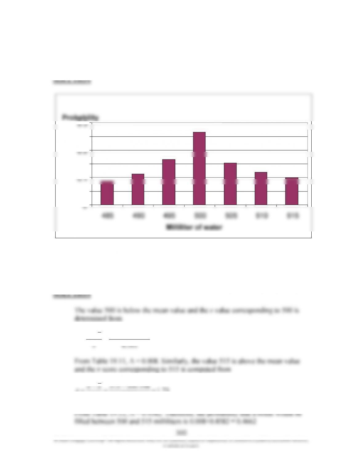
19.34 For Problem 19.33, calculate the probability distribution and plot the probability
distribution curve.
19.35 For Problem 19.33, determine the probability (assuming normal distribution) that
a bottle would be filled between 500 and 515 milliliters.
02.0
561
.
8
198.500500
s
xx
z
0
0.05
0.15
0.25
0.3
485 490 495
500 505 510 515
Milliliter of water
Probability
361
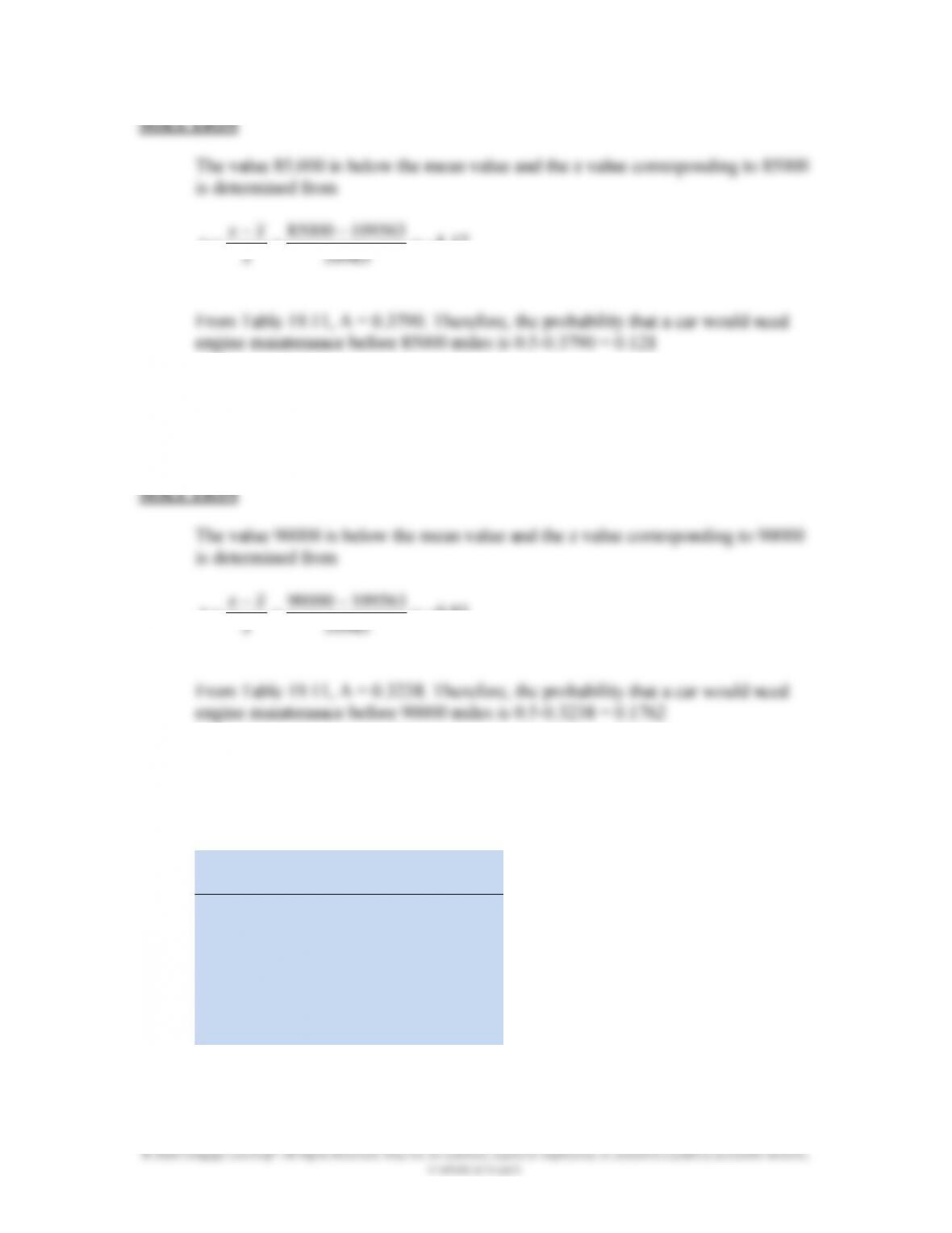
19.36 For Problem 19.33 determine the probability (assuming normal distribution) that a
bottle would be filled with more than 495 milliliters.
61.0
561
.
8
198.500495
s
xx
z
19.37 For Problem 19.33, determine the probability (assuming normal distribution) that
a bottle would be filled with less than 500 milliliters.
02.0
561
.
8
198.500500
s
xx
z
19.38 For Problem 19.33, determine the probability (assuming normal distribution) that
a bottle would be filled with less than 495 milliliters.
362
© 2020 Cengage Learning®. All Rights Reserved. May not be scanned, copied or duplicated, or posted to a publicly accessible website,
in whole or in part.
SOLUTION
The value 495 is below the mean value and the z value corresponding to 495 is
determined from
61.0
561
.
8
198.500495
s
xx
z
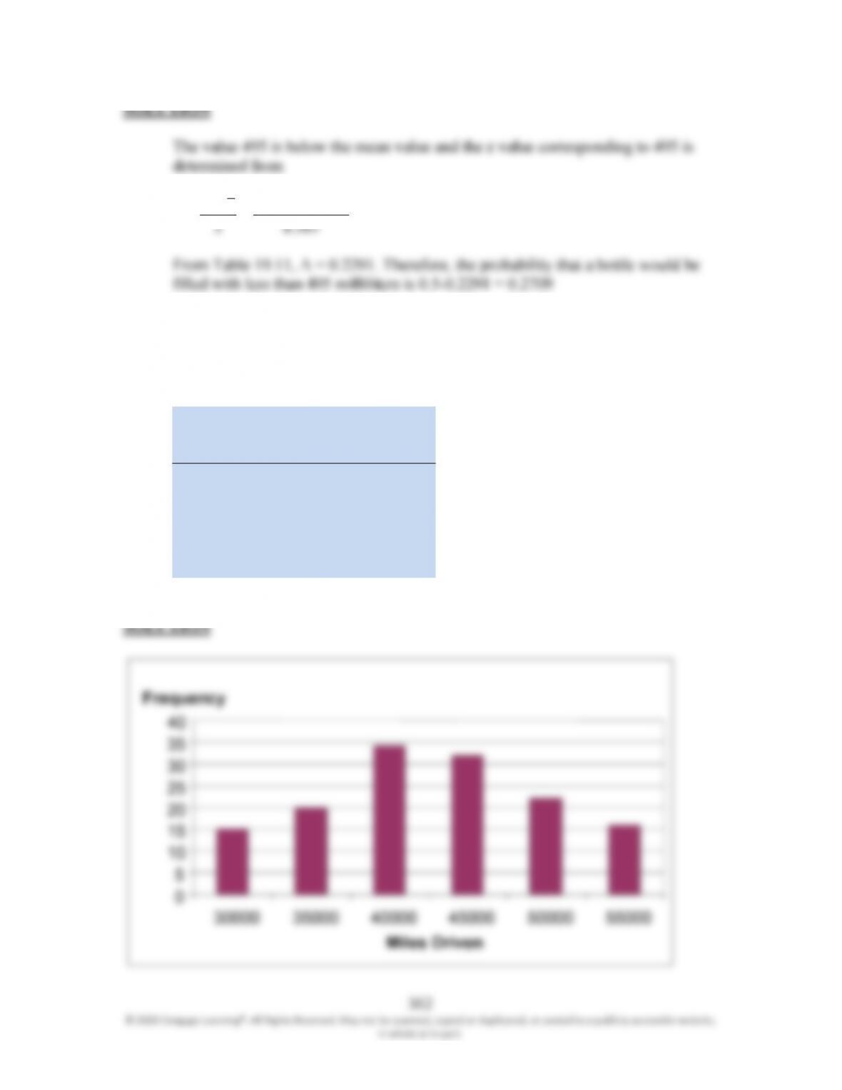
19.39 As a chemical engineer working for a tire manufacturer, you collect the following
data in order to test the performance of tires. Plot the data and calculate the mean
and standard deviation.
Miles with
Acceptable
(Reliable) Wear Frequency
30,000
15
35,000
20
40,000
34
45,000
32
50,000
22
55,000
16
0
5
10
15
20
25
30
35
40
30000
35000 40000 45000 50000
55000
Miles Driven
363
© 2020 Cengage Learning®. All Rights Reserved. May not be scanned, copied or duplicated, or posted to a publicly accessible website,
in whole or in part.
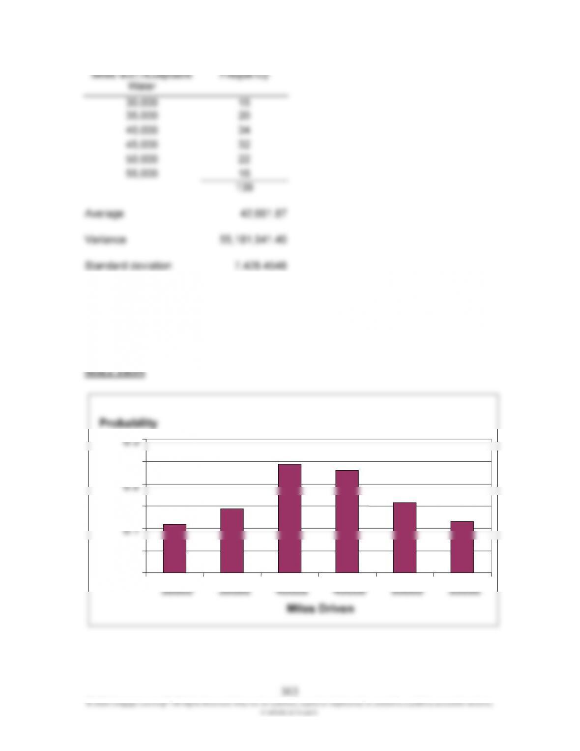
Miles with Acceptable
Water
Frequency
42,661.87
55,181,941.40
19.40 For Problem 19.39, calculate the probability distribution and plot the probability
distribution curve.
364
19.41 For Problem 19.39, determine the probability (assuming normal distribution) that
a tire could be used reliably between 45,000 and 55,000 miles.
31.0
45
.
7428
87.4266145000
s
xx
z
66.1
45
.
7428
87.4266155000
s
xx
z
19.42 For Problem 19.39, determine the probability (assuming normal distribution) that
a tire could be used reliably for more than 50,000 miles.
99.0
45
.
7428
87.4266150000
s
xx
z
19.43 For Problem 19.39, determine the probability (assuming normal distribution) that
a tire could be used reliably for less than 45,000 miles.
365
© 2020 Cengage Learning®. All Rights Reserved. May not be scanned, copied or duplicated, or posted to a publicly accessible website,
in whole or in part.
SOLUTION
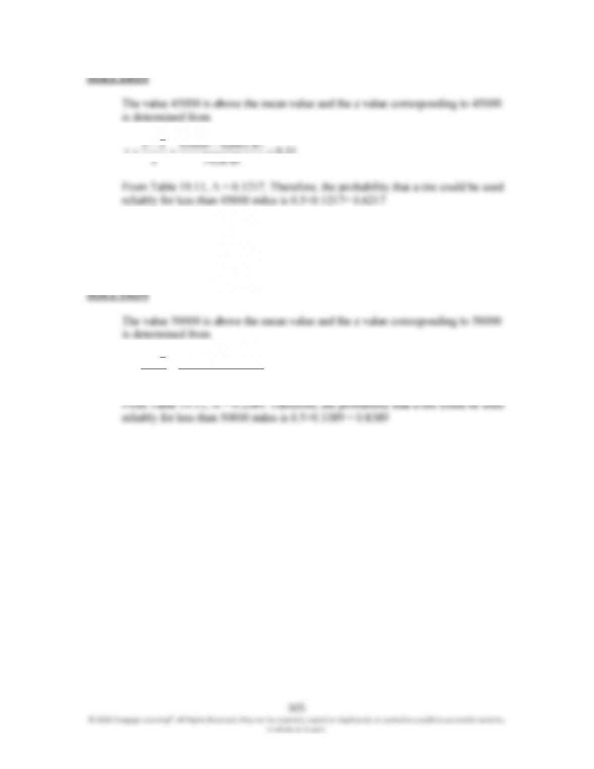
The value 45000 is above the mean value and the z value corresponding to 45000
is determined from
31.0
45
.
7428
s
z
19.44 For Problem 19.39, determine the probability (assuming normal distribution) that
a tire could be used reliably for less than 50,000 miles.
99.0
45
.
7428
87.4266150000
s
xx
z