Civil Engineering Chapter 18 Given The Following Matrices And Calculate The Determinant And Direct Expansion Which

322

18.18 Given the following matrices:

 

















18412

14616

0102

Aand

 

















18412

0204

0102

B ,

calculate the determinant of [A] and [B] by direct expansion. Which matrix is singular?

18.19 Solve the following set of equations using the Gaussian method.

2x + 6 y = 28 (1)

8 x + 2y = 2 (2)

SOLUTION

323

in whole or in part.

Substitute y = 5 in Eq. (1), to solve for x:

x = 14 – 3(5)  x = -1

18.20 Solve the following set of equations using the Gaussian method.

-6 x1 + 9 x2 = 15 (1)

x1 + x2 = 10 (2)

18.21 Solve the following set of equations using the Gaussian method.

2 2 2

2 5 1

-9 3 15x1

x2

x3=12

15

42



 

324

in whole or in part.























































14

15

6

513

152

111

3

2

1

x

or (3) 1453

(2) 1552

(1) 6

321









xxx

Multiply Eq. (1) by -2 and add to Eq. (2):

(4) 33

1552

12222

32

321













xx

xxx

Multiply Eq. (1) by 3 and add to Eq. (3):

(5) 3284

1453

18333

32

321











xx

xxx

Multiply Eq. (4) by -4/3 and add to Eq. (5):

3 28 28/3

–––––––––––––––––––––––––––

3284

43/44

33

32













xx

and by back substitution we find: x2 = 2 and x1 =1.

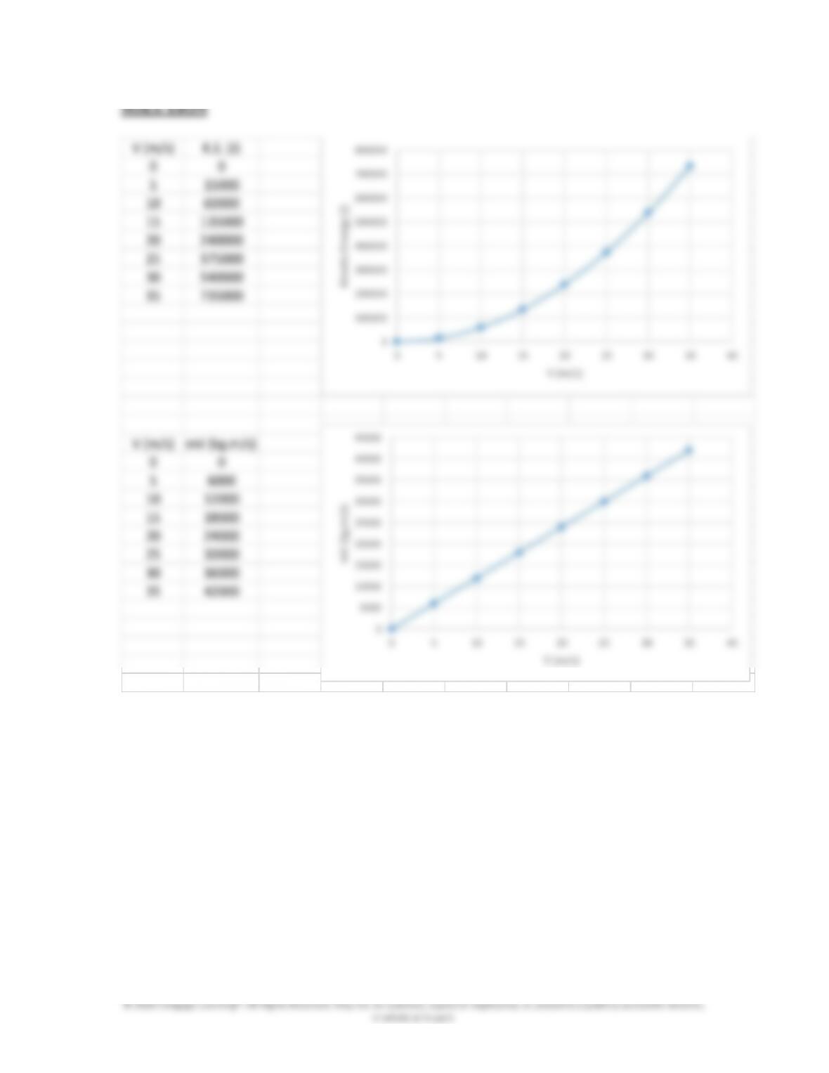
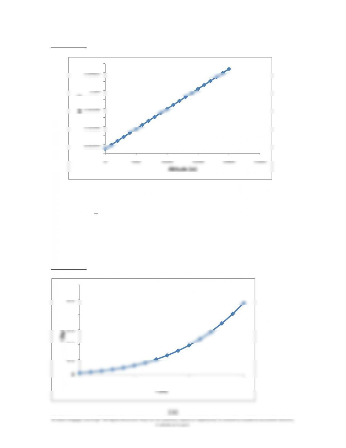
18.22 As we explained in Chapter 13, an object having a mass m and moving with a

speed V has a kinetic energy, which is equal to

kinetic energy = 1

2 𝑚𝑉

Plot the kinetic energy of a car with a mass of 1200 kg as the function of its

speed. Vary

the speed from zero to 35 m/s (126 km/h). Determine the rate of change of kinetic

energy of the car as a function of speed and plot it. What does this rate of change

represent?

325

in whole or in part.

SOLUTION

18.23 In Chapter 13, we explained that when a spring is stretched or compressed from its

stretched position, elastic energy is stored in the spring, and that energy will be

released when the spring is allowed to return to its unstretched position. The elastic

energy stored in a spring when stretched or compressed is determined from:





x

FdxEnergyElastic

0

Obtain expressions for the elastic energy of a linear spring described by

F = k x and a hard spring whose behavior is described by F = k x2.

326

in whole or in part.

SOLUTION

For a linear spring:

2

00 2

1

Energy Elastic kxkxdxFdx

xx

 

For a hard spring:

3

0

2

03

1

Energy Elastic kxdxkxFdx

xx

 

18.24 For Example 1 in Table 18.8, verify that the given solution satisfies the governing

differential equation and the boundary conditions.

SOLUTION

327

18.25 For Example 3 in Table 18.8, verify that the given solution satisfies the governing

differential equation and the initial conditions.

SOLUTION

kA

c

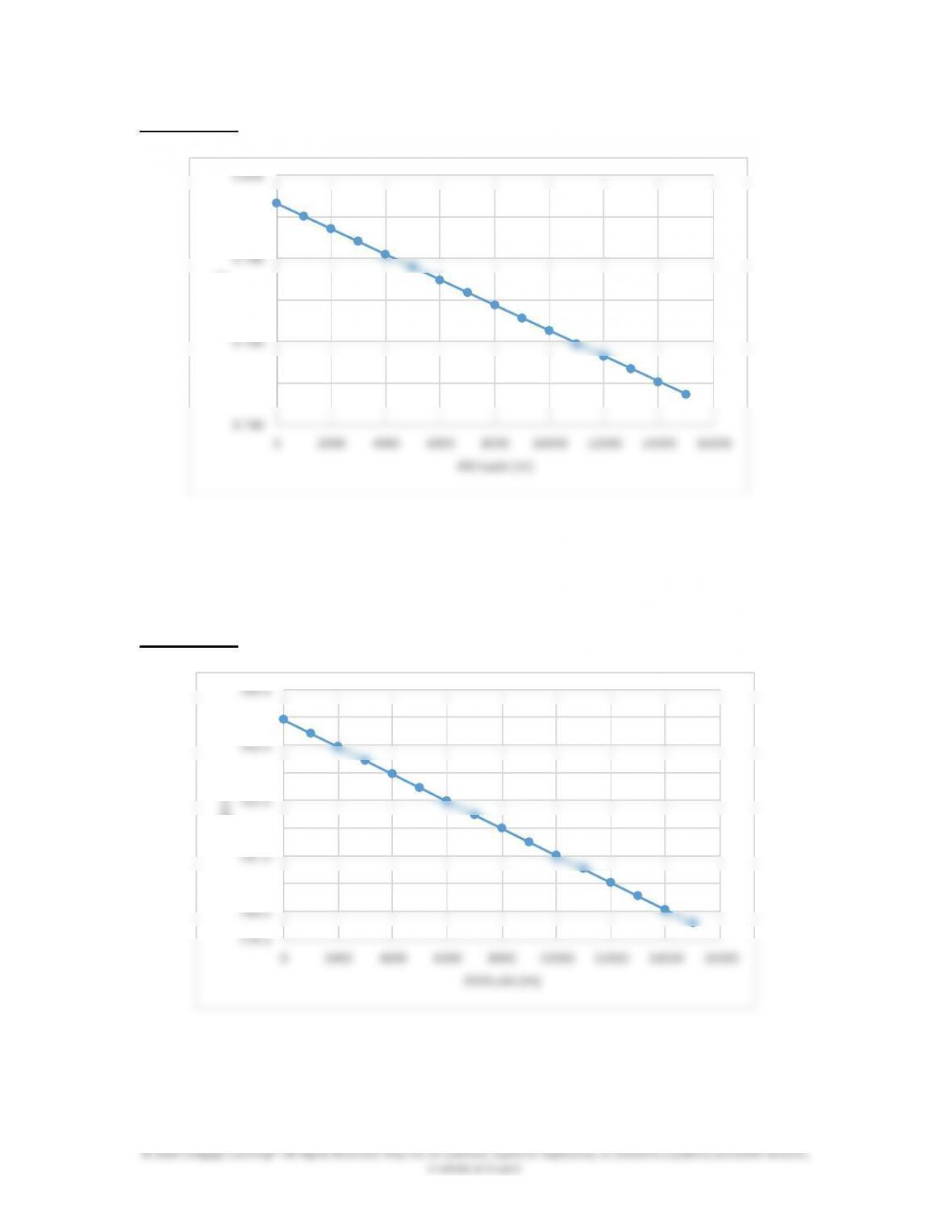
18.26 We presented Newton’s Law of Gravitation in Chapter 10. We also explained the

acceleration due to gravity. Create a graph that shows the acceleration due to

gravity as a function of distance from the earth’s surface. Change the distance

from sea level to an altitude of 15,000 m.

328

SOLUTION

329

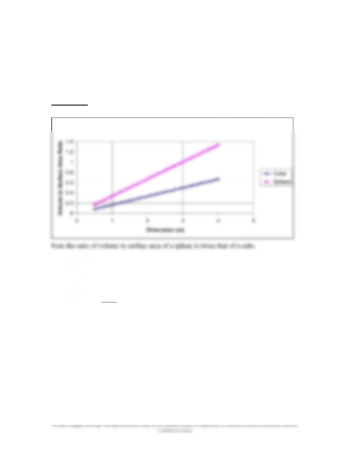
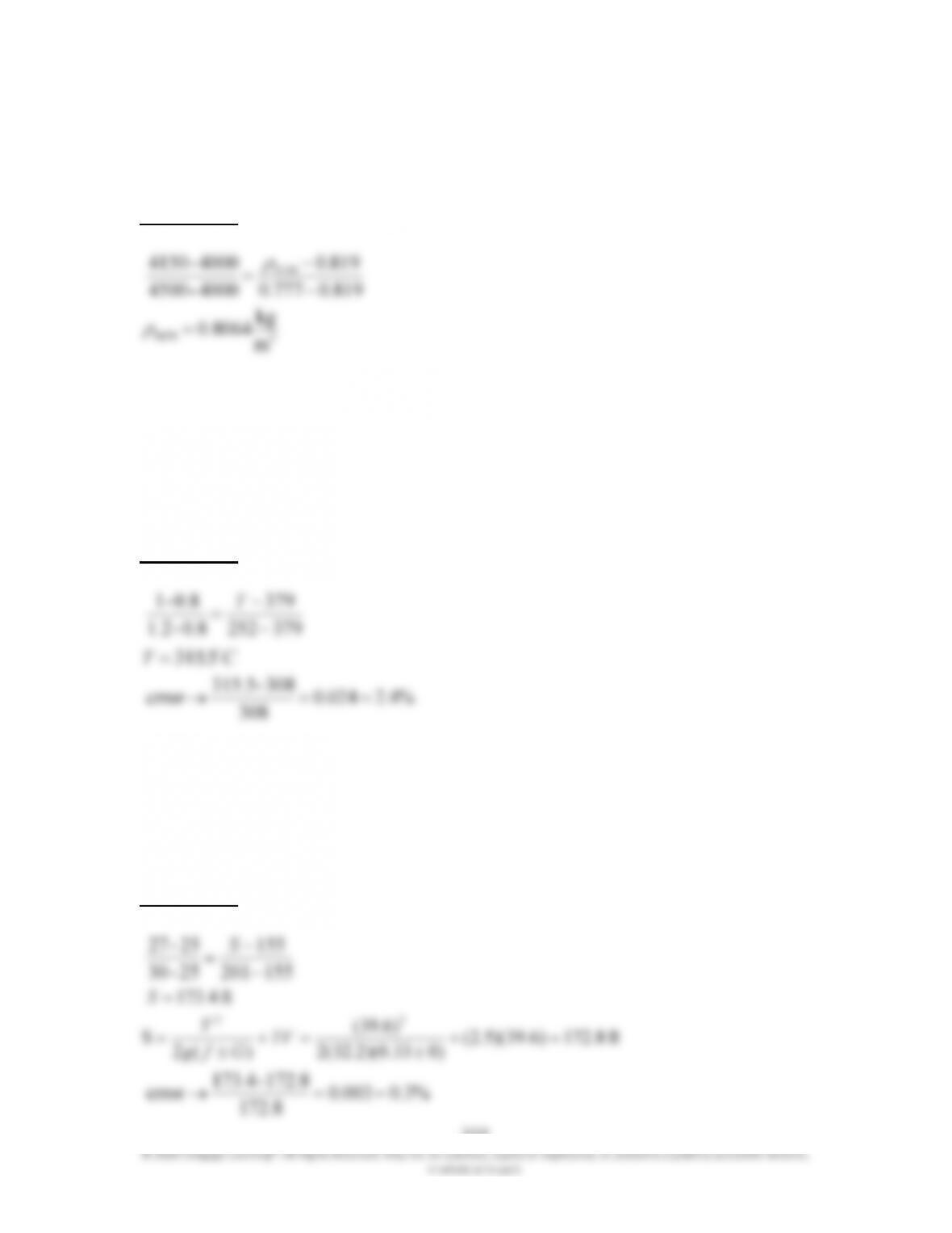
18.28 An engineer is considering storing some radioactive material in a container she is

creating. As a part of her design, she needs to evaluate the ratio of volume to

surface area of two storage containers. Create curves that show the ratio of

volume to surface area of a sphere and a square container. Create another graph

that shows the difference in the ratios. Vary the radius or the side dimension of a

square container from 50 cm to 4 m.

SOLUTION

18.29 As we mentioned in Chapter 10, engineers used to use pendulums to measure the

value of g at a location. The formula to use the measure the acceleration due to

gravity is

𝑔=4𝜋𝐿

𝑇

where g is acceleration due to gravity (m/s2), L is the length of pendulum, and T is

the period of oscillation of the pendulum (the time that it takes the pendulum to

complete one cycle). For a pendulum of 2 m long, create a graph that could be

used for locations between an altitude of 0 and 2000 m, and shows g as a function

of T.

Volume to Surface Area Ratios vs Side/Radius Dimension

0

0.2

0.4

0.6

0.8

1

1.2

1.4

0 1 2 3 4 5

Dimension (m)

Volume to Surface Area Ratio

Cube

Sphere

SOLUTION

2.8393

2.8395

2.8397

2.8399

2.8401

2.8403

T (seconds)

331

18.31 Use the linear interpolation method discussed in Section 18.2 to estimate the

density of air at an altitude 4150 m.

SOLUTION

819

.

0

777

.

0

4000

–

4500



3

4150

m

18.32 For the cooling of steel plates discussed in Section 18.4 (Figure 18.17) using

linear interpolation, estimate the temperature of the plate at time equal to 1 hr,

from the temperature data at 0.8 hr and 1.2 hour. Compare the estimated

temperature value to the actual value of 308°C. What is the percentage of error?

SOLUTION

379

252

0.8

–

1.2



308

18.33 For the stopping sight distance problem of Figure 18.12, estimate the stopping

distance for speed of 27 mph, using the 25 mph and 30 mph data. Compare the

estimated stopping distance value to the actual value from Equation (18.7). What

is the percentage of error?

SOLUTION

155

201

155

25

–

30

25–27



S

ft 173.4



S

ft 172.8)6.39)(5.2(

)033.0)(2.32(2

)6.39(

)(2

S

22









TV

Gfg

V

%3.0003.0

172.8

172.8–173.4

error 

332

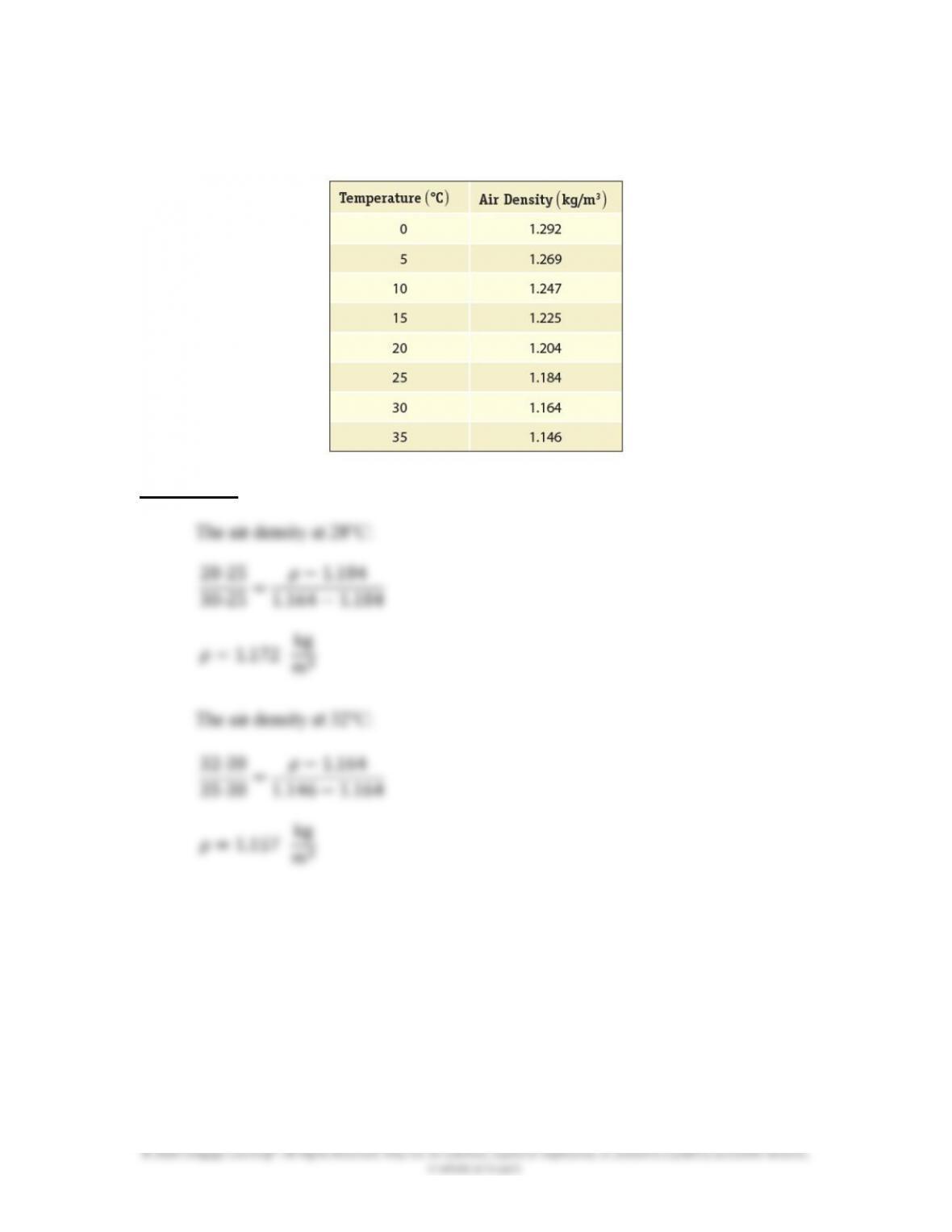
18.34 The variation of air density at the standard pressure as a function of temperature is

given in the accompanying table. Use linear interpolation to estimate the air

density at 28℃ and 32℃.

SOLUTION

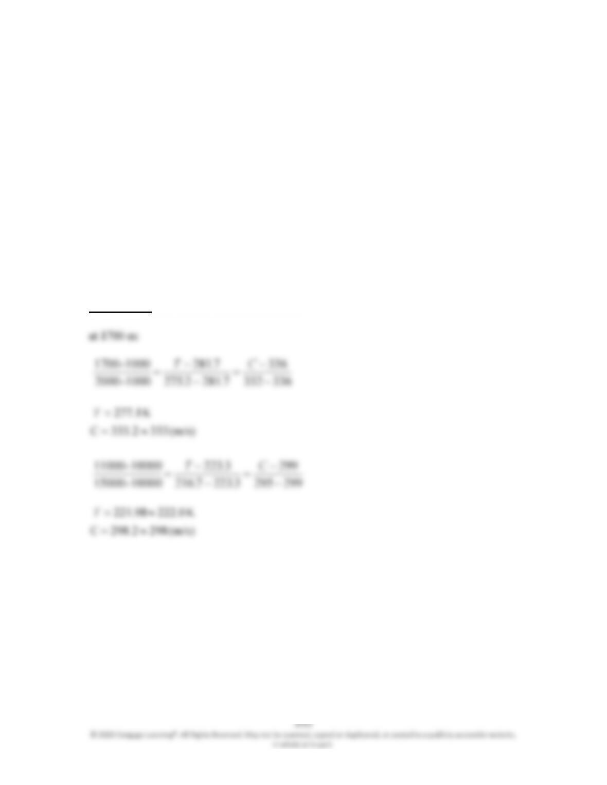
18.35 The air temperature and speed of sound for the U.S. standard atmosphere is given

in the accompanying table. Using linear interpolation, estimate the air

temperatures and the corresponding speeds of sound at altitudes of 1700 m and

11,000 m.

Altitude (m)

Air Temperature (K) Speed of Sound (m/s)

500 284.9 338

1,000 281.7 336

2,000 275.2 332

5,000 255.7 320

10,000 223.3 299

15,000 216.7 295

20,000 216.7 295

SOLUTION

(m/s) 298298.2C



334

in whole or in part.

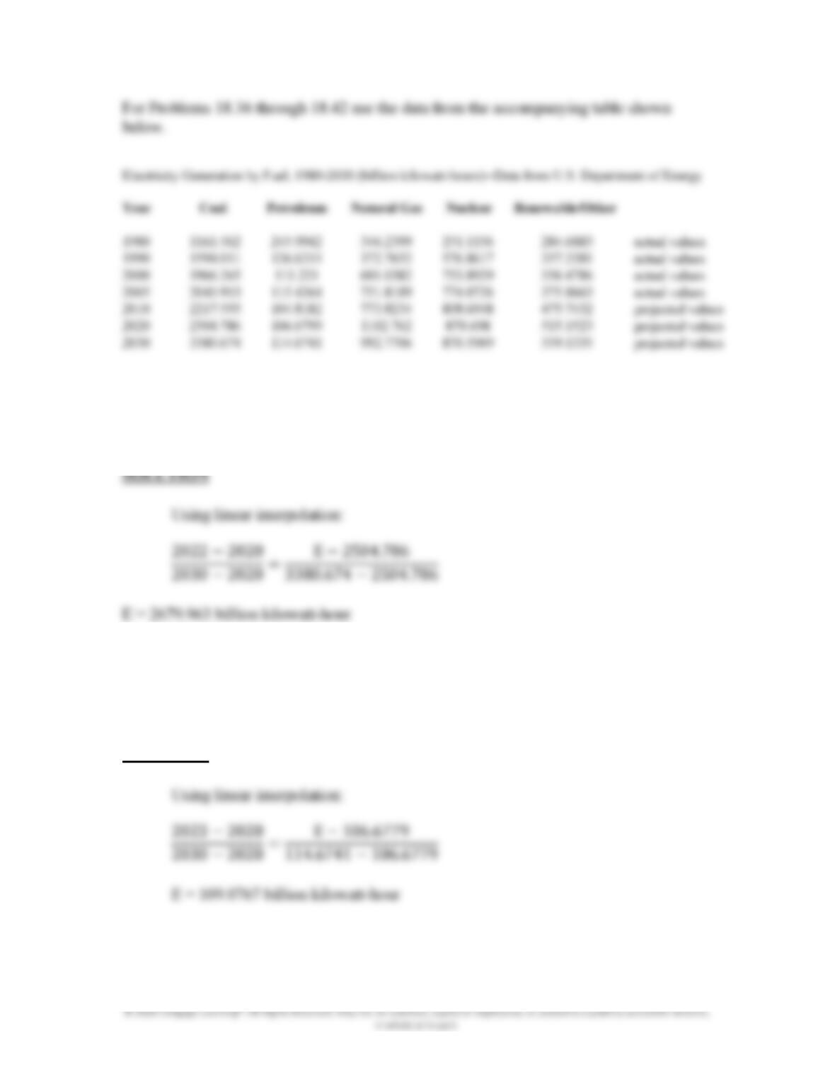
For Problems 18.36 through 18.42 use the data from the accompanying table shown

below.

Electricity Generation by Fuel, 1980

–

2030 (billion kilowatt

–

hours)

—

Data from U.S. Department of Energy

Year Coal Petroleum Natural Gas Nuclear Renewable/Other

1980 1161.562 245.9942 346.2399 251.1156 284.6883 actual values

1990 1594.011 126.6211 372.7652 576.8617 357.2381 actual values

2000 1966.265 111.221 601.0382 753.8929 356.4786 actual values

2005 2040.913 115.4264 751.8189 774.0726 375.8663 actual values

2010 2217.555 104.8182 773.8234 808.6948 475.7432 projected values

2020 2504.786 106.6799 1102.762 870.698 515.1523 projected values

2030 3380.674 114.6741 992.7706 870.5909 559.1335 projected values

18.36 Estimate the amount of electricity that is projected to be generated from coal in

2022.

18.37 Estimate the amount of electricity that is projected to be generated from

petroleum in 2023.

SOLUTION

335

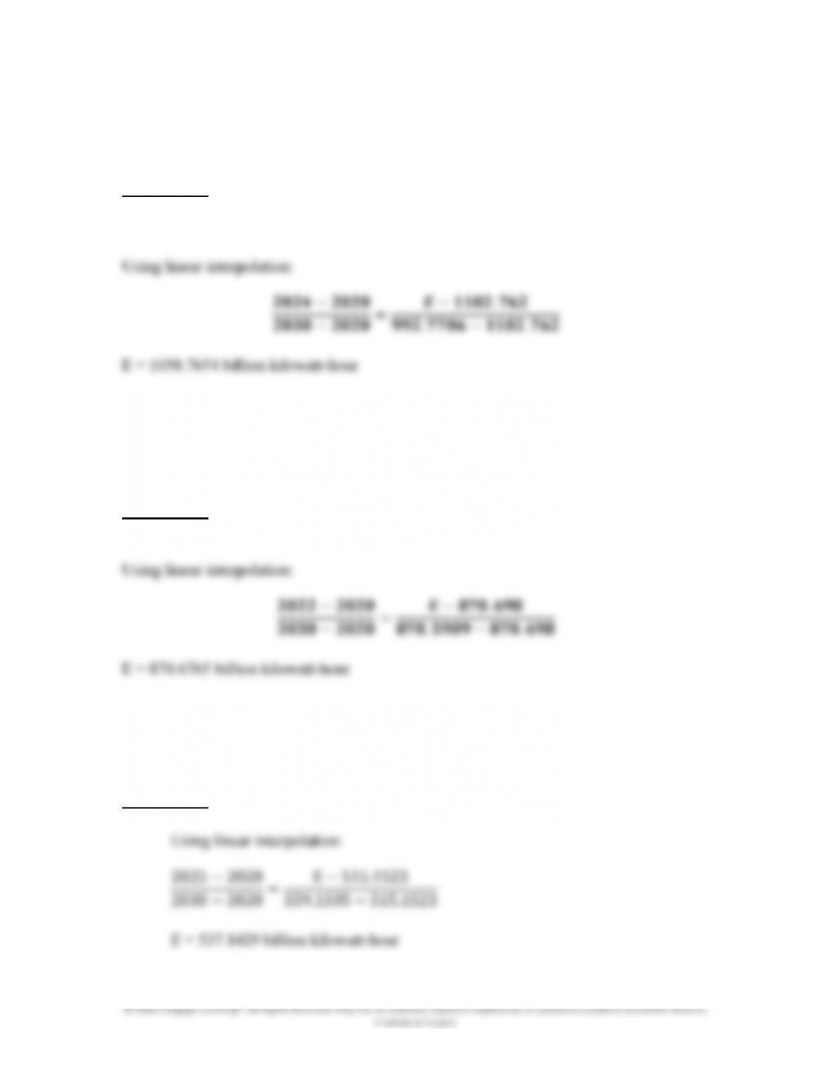
18.38 Estimate the amount of electricity that is projected to be generated from natural

gas in 2024.

SOLUTION

18.39 Estimate the amount of electricity that is projected to be generated from nuclear

fuel in 2022.

SOLUTION

18.40 Estimate the amount of electricity that is projected to be generated from

renewable and other sources in 2025.

SOLUTION

336

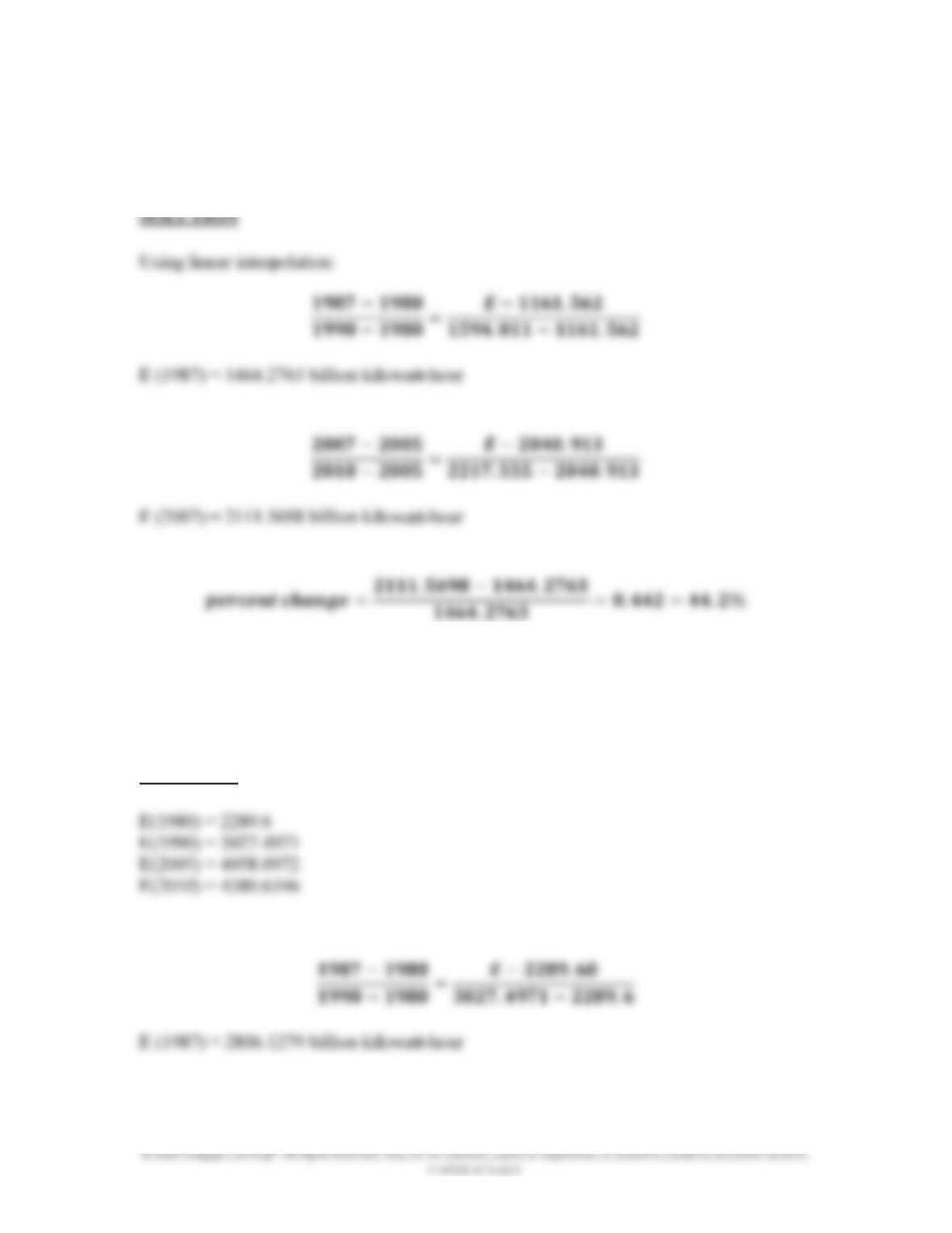
18.41 Using linear interpolation, estimate the percentage change in the amount of

electricity that was generated using coal in 2007 compared to 1987.

18.42 Using linear interpolation, estimate the percentage change in the total amount of

electricity that was generated in 2007 compared to 1987.

SOLUTION

337

in whole or in part.

𝟐𝟎𝟎𝟕−𝟐𝟎𝟎𝟓

𝟐𝟎𝟏𝟎−𝟐𝟎𝟎𝟓=𝑬−𝟒𝟎𝟓𝟖.𝟎𝟗𝟕𝟐

𝟒𝟑𝟖𝟎,𝟔𝟑𝟒𝟔−𝟒𝟎𝟓𝟖.𝟎𝟗𝟕𝟐

E (2007) = 4187.1121 billion kilowatt-hour

𝒑𝒆𝒓𝒄𝒆𝒏𝒕 𝒄𝒉𝒂𝒏𝒈𝒆=𝟒𝟏𝟖𝟕,𝟏𝟏𝟐𝟏−𝟐𝟖𝟎𝟔.𝟏𝟐𝟕𝟗

𝟐𝟖𝟎𝟔.𝟏𝟐𝟕𝟗 =𝟎.𝟒𝟗𝟐=𝟒𝟗.𝟐%