16-1
CHAPTER 16. BAYESIAN METHODS
CHAPTER 16. BAYESIAN METHODS …………………………….…………………………………………………1
16.1. Introduction ……………………………………………………………………………………………..……………..1
16.2. Bayesian Probabilities …………………………………………………………………………………….………..1
16.3. Bayesian Estimation of Parameters …………………………………………………………………………....8
16.4. Bayesian Statistics ……………………………………………………………………………………….…………..8
The following table provides a summary of the problems with their appropriate sections:
Section Problems
16.1 None
16.1. Introduction
None
16.2. Bayesian Probabilities
Problem 16-1.
The following probabilities as given in the problem and the figure below can be used to compute
the average as a weighted value:
p P(p)
0.1 0.3
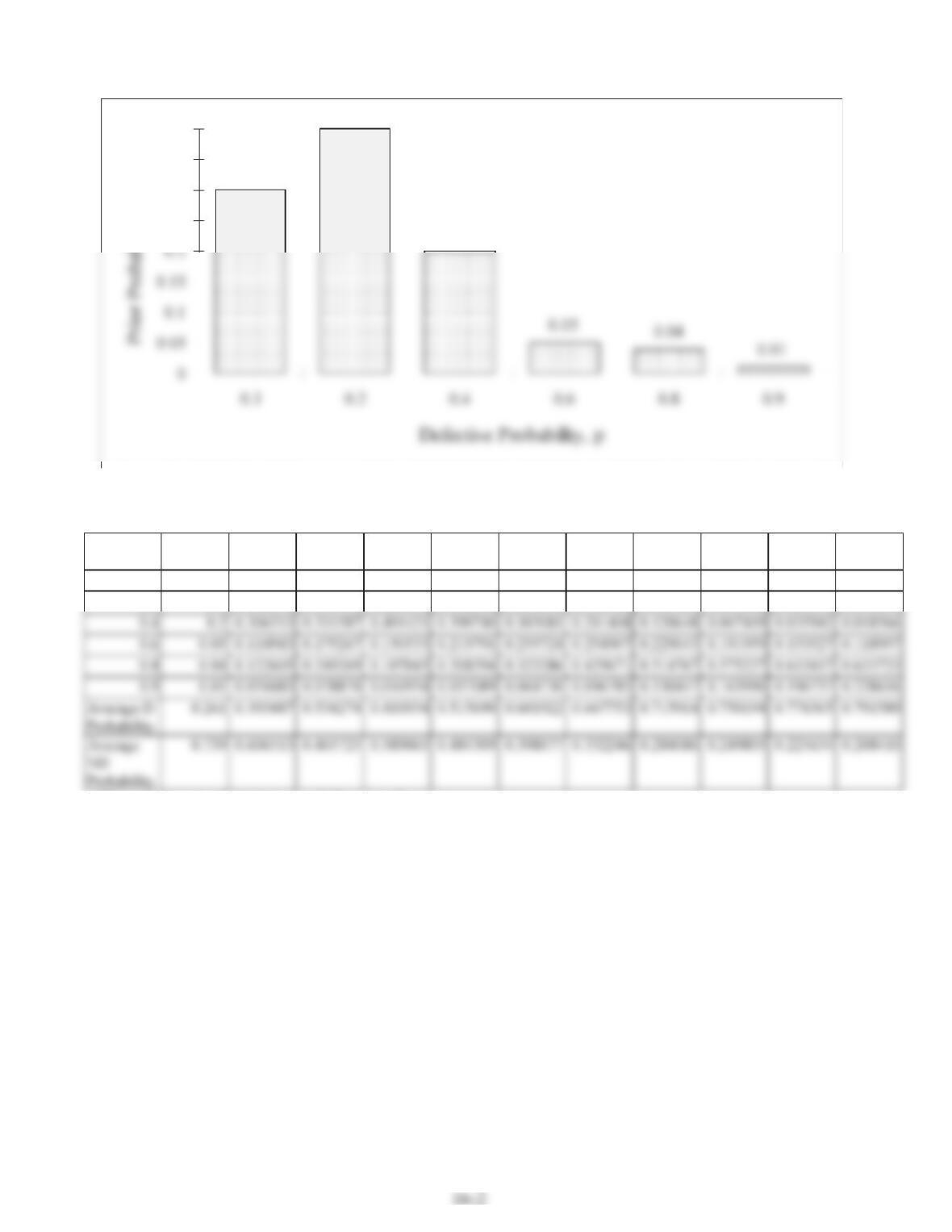
The following posterior probabilities and averages can be computed as required for parts b, c, d, e
and f of the problem:
p P(p) Post. 1 D Post. 2 D Post. 3
ND
Post. 4 D Post. 5 D Post. 6 D Post. 7 D Post. 8 D Post. 9 D Post. 10
D
0.1 0.3 0.114943 0.029211 0.056449 0.013737 0.002663 0.000442 6.62E-05 9.25E-06 1.2E-06 1.59E-07
0.2 0.4 0.306513 0.155793 0.267614 0.130246 0.050513 0.016784 0.005027 0.001404 0.000374 9.67E-05
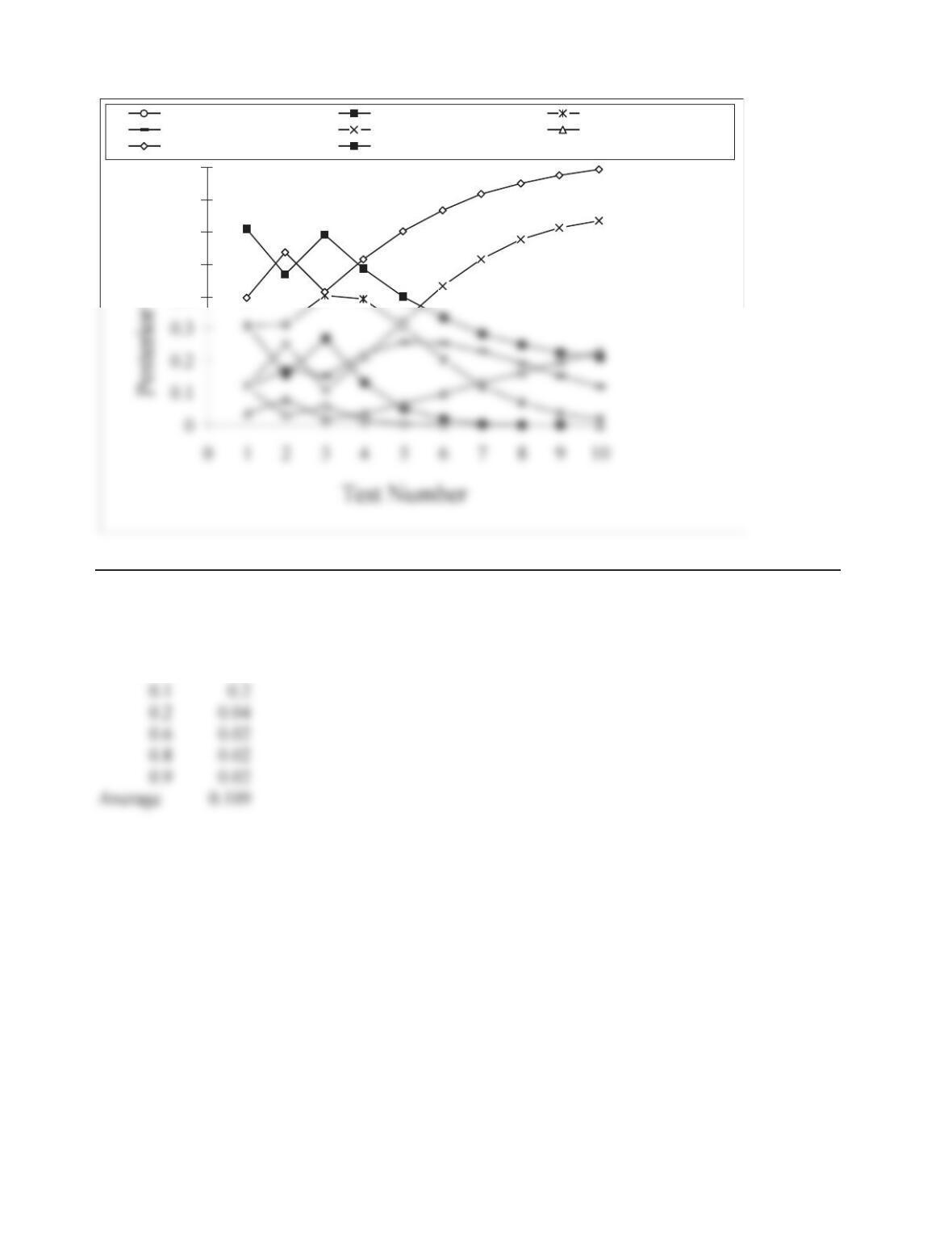
The results are plotted in the following figure:
0.3
0.4
0.2
0.25
0.3
0.35
0.4
16-3
Problem 16-2.
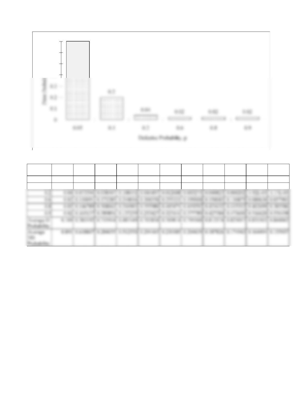
The following probabilities as given in the problem and the figure below can be used to compute
the average as a weighted value:
p P(p)
0.05 0.7
0.4
0.5
0.6
0.7
0.8
0.1 0.2 0.4
0.6 0.8 0.9
Average D Probability Average ND Probability
16-4
The following posterior probabilities and averages can be computed as required for parts b, c, d, e
and f of the problem:
p P(p) Post. 1 D Post. 2 D Post. 3
ND
Post. 4 D Post. 5 D Post. 6 D Post. 7 D Post. 8 D Post. 9 D Post. 10
D
0. 0.7 0.321100 0.042117 0.14086 0.014448 0.001023 6.65E-05 4.18E-06 2.57E-07 1.56E-08 9.33E-10
0.1 0.2 0.183486 0.048134 0.152510 0.031287 0.004432 0.000575 7.24E-05 8.91E-06 1.08E-06 1.29E-07
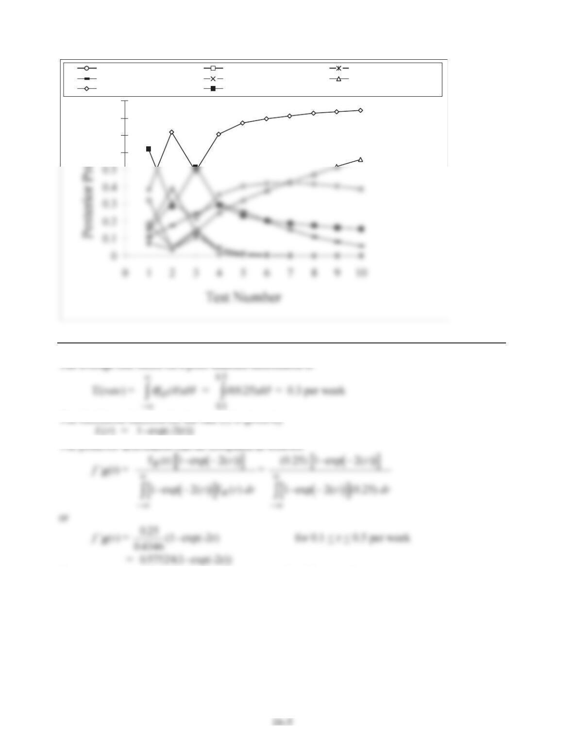
The results are plotted in the following figure:
0.7
0.4
0.5
0.6
0.7
p
Problem 16-3.
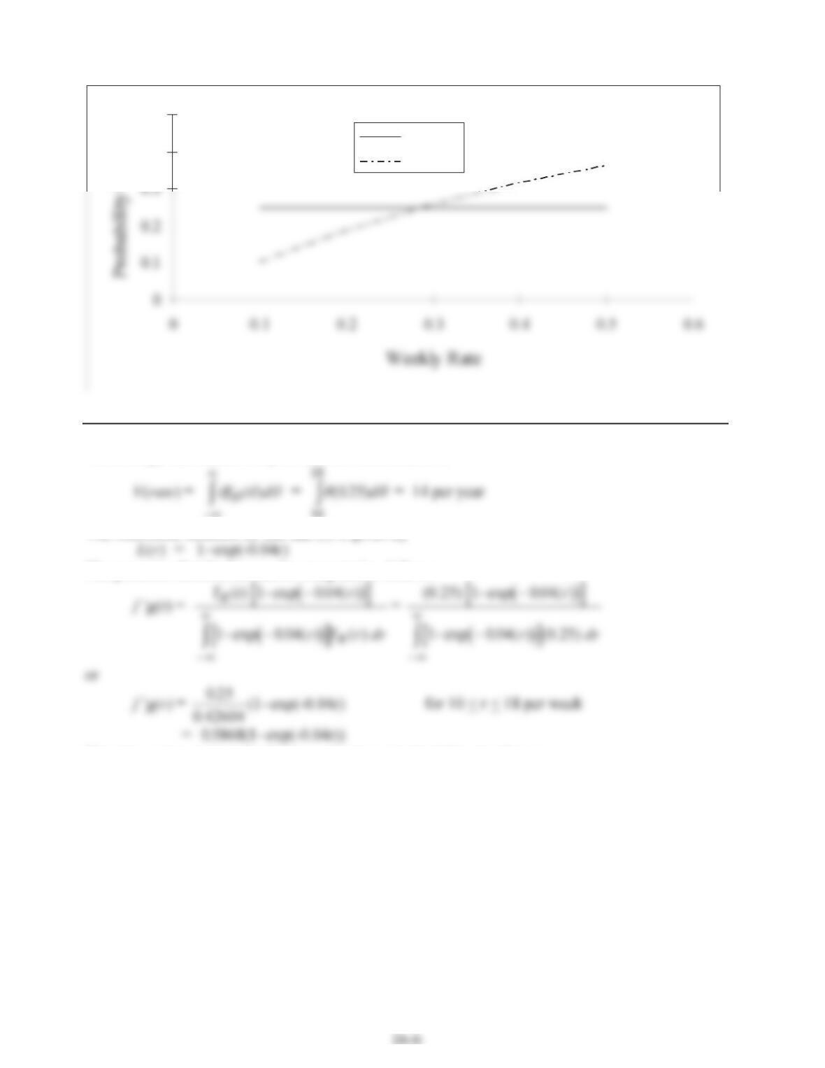
The prior and posterior distributions are shown in the following figure:
0.6
0.7
0.8
0.9
0.1 0.2 0.4
0.6 0.8 0.9
Average D Probability Average ND Probability
Problem 16-4.
The average rate based on a prior uniform distribution is
f
10
The likelihood function for the rate (r) is given by
The posterior distribution can be computed as follows:
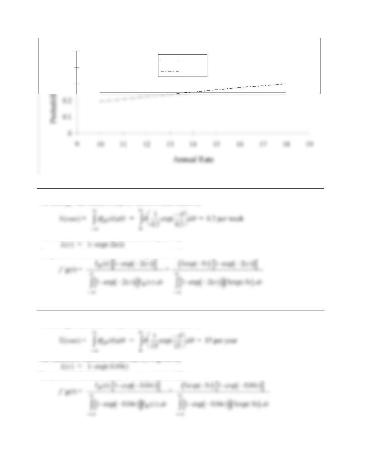
The prior and posterior distributions are shown in the following figure:
0.4
0.5
y
Prior
Posterior
16-7
Problem 16-5.
The average rate based on a prior uniform distribution is
The likelihood function for the rate (r) is given by
The posterior distribution can be computed as follows:
Problem 16-6.
The average rate based on a prior uniform distribution is
The posterior distribution can be computed as follows:
0.3
0.4
0.5
y
Prior
Posterior
16-8
16.3. Bayesian Estimation of Parameters
Problems 16-1 to 16-6 (refer to Section 16.2).
16.4. Bayesian Statistics
Problem 16-7.
The information provided in the problem can be used to update the prior mean and variance of the
average thickness using Eqs. 16-42 as follows:
Therefore, the posterior standard deviation is 0.4340 mm. The prior mean value and variance can
be used to establish the following prior 95% confidence interval on the mean (using Eq. 16-43a):
Problem 16-8.
The information provided in the problem can be used to update the prior mean and variance of the
average thickness using Eqs. 16-42 as follows:
Therefore, the posterior standard deviation is 0.2041 mm. The prior mean value and variance can
be used to establish the following prior 95% confidence interval on the mean (using Eq. 16-43a):
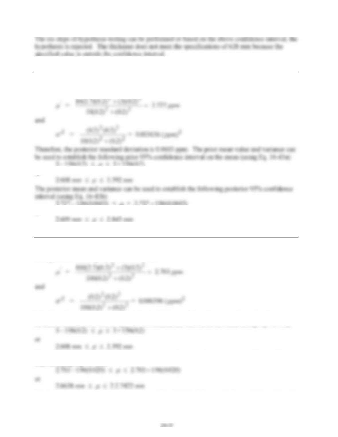
Problem 16-9.
The information provided in the problem can be used to update the prior mean and variance of the
average thickness using Eqs. 16-42 as follows:
or
2 727 196 0 0603 196 0 0603. . (. ) . (. )
dd 2.727
P
or
Problem 16-10.
The information provided in the problem can be used to update the prior mean and variance of the
average thickness using Eqs. 16-42 as follows:
Therefore, the posterior standard deviation is 0.020 ppm. The prior mean value and variance can
be used to establish the following prior 95% confidence interval on the mean (using Eq. 16-43a):
The posterior mean and variance can be used to establish the following posterior 95% confidence
interval (using Eq. 16-43b):
The larger sample size with the same mean and standard deviation results in a confidence interval
with a smaller width due to primarily a smaller posterior standard deviation for the mean.