225
x
L
w
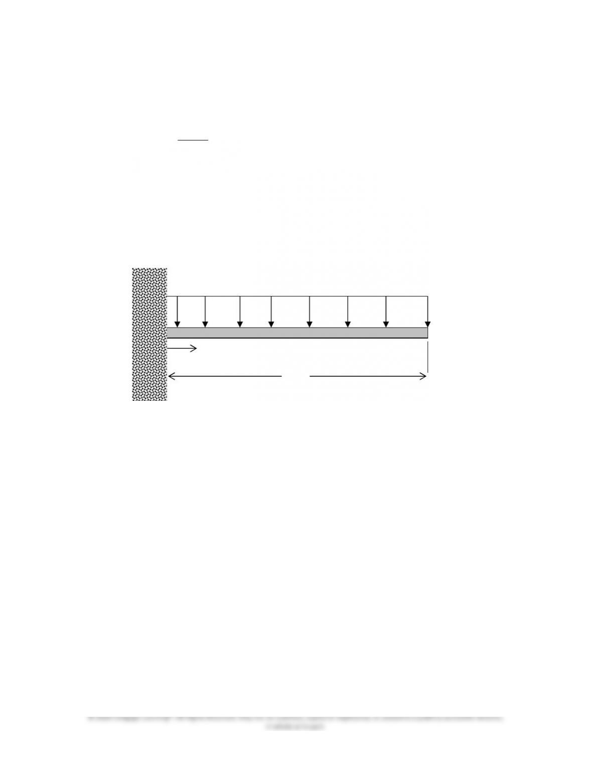
15.11 The cantilevered beam shown in the accompanying figure is used to support a
load acting on a balcony. The deflection of the centerline of the beam is given by
the following equation
)64(
24
22
2
LLxx
EI
wx
y
where
y = deflection at a given x location (m)
w = distributed load (N/m)
E = modulus of elasticity (N/m2)
I = second moment of area (m4)
x = distance from the support as shown (m)
L = length of the beam (m)
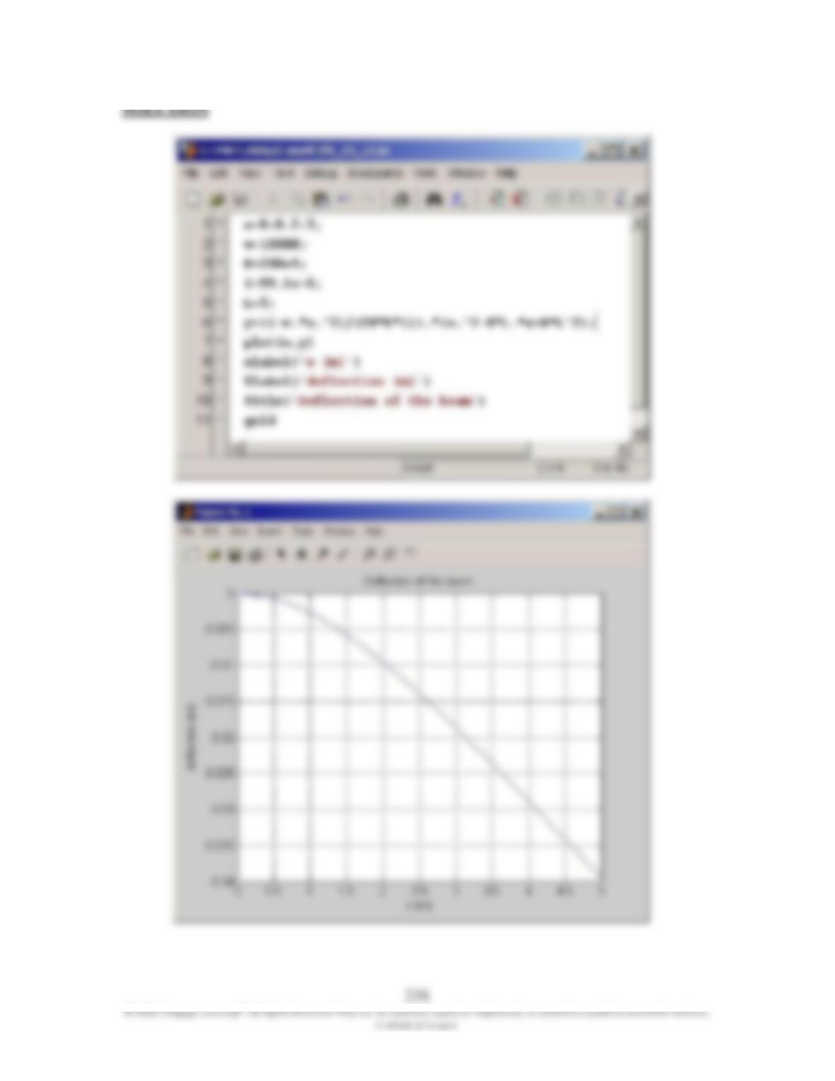
Using MATLAB, plot the deflection of a beam whose length is 5 m with the
modulus of elasticity of E = 200 GPa and I = 99.1 x 106 mm4. The beam is
designed to carry a load of 10000 N/m. What is the maximum deflection of the
beam?
226
© 2020 Cengage Learning®. All Rights Reserved. May not be scanned, copied or duplicated, or posted to a publicly accessible website,
in whole or in part.
SOLUTION

227
15.12 Fins, or extended surfaces, are commonly used in a variety of engineering
applications to enhance cooling. Common examples include a motorcycle engine
head, a lawn mower engine head, extended surfaces used in electronic equipment,
and finned tube heat exchangers in room heating and cooling applications.
Consider aluminum fins of a rectangular profile shown in Problem 14.13, which
are used to remove heat from a surface whose temperature is 100C. The
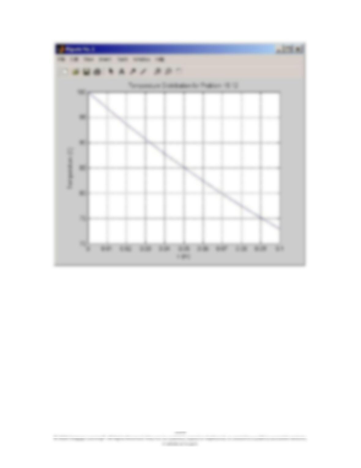
temperature of the ambient air is 20C. We are interested in determining how
the temperature of the fin varies along its length and plotting this temperature
variation. For long fins, the temperature distribution along the fin is given by:
mx
ambientbaseambient eTTTT
)(
where
kA
hp
m
and
h = the heat transfer coefficient (W/m2·K)
p = perimeter 2* (a + b) of the fin (m)
A = cross-sectional area of the fin (a*b) (m2)
k = thermal conductivity of the fin material (W/m·K)
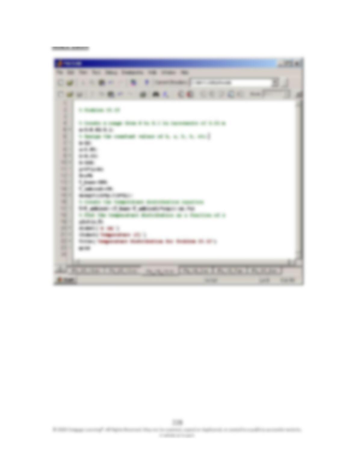
Plot the temperature distribution along the fin using the following data:
k = 168 W/m·K, h = 12 W/m2·K, a = 0.05 m, b = 0.01 m. Vary x from 0 to 0.1 m
in increments of 0.01 m.
228
© 2020 Cengage Learning®. All Rights Reserved. May not be scanned, copied or duplicated, or posted to a publicly accessible website,
in whole or in part.
SOLUTION
229
© 2020 Cengage Learning®. All Rights Reserved. May not be scanned, copied or duplicated, or posted to a publicly accessible website,
in whole or in part.
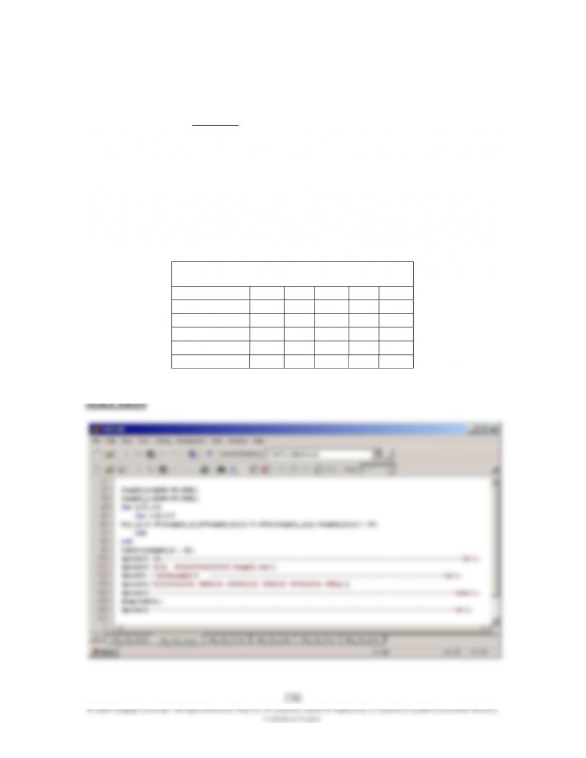
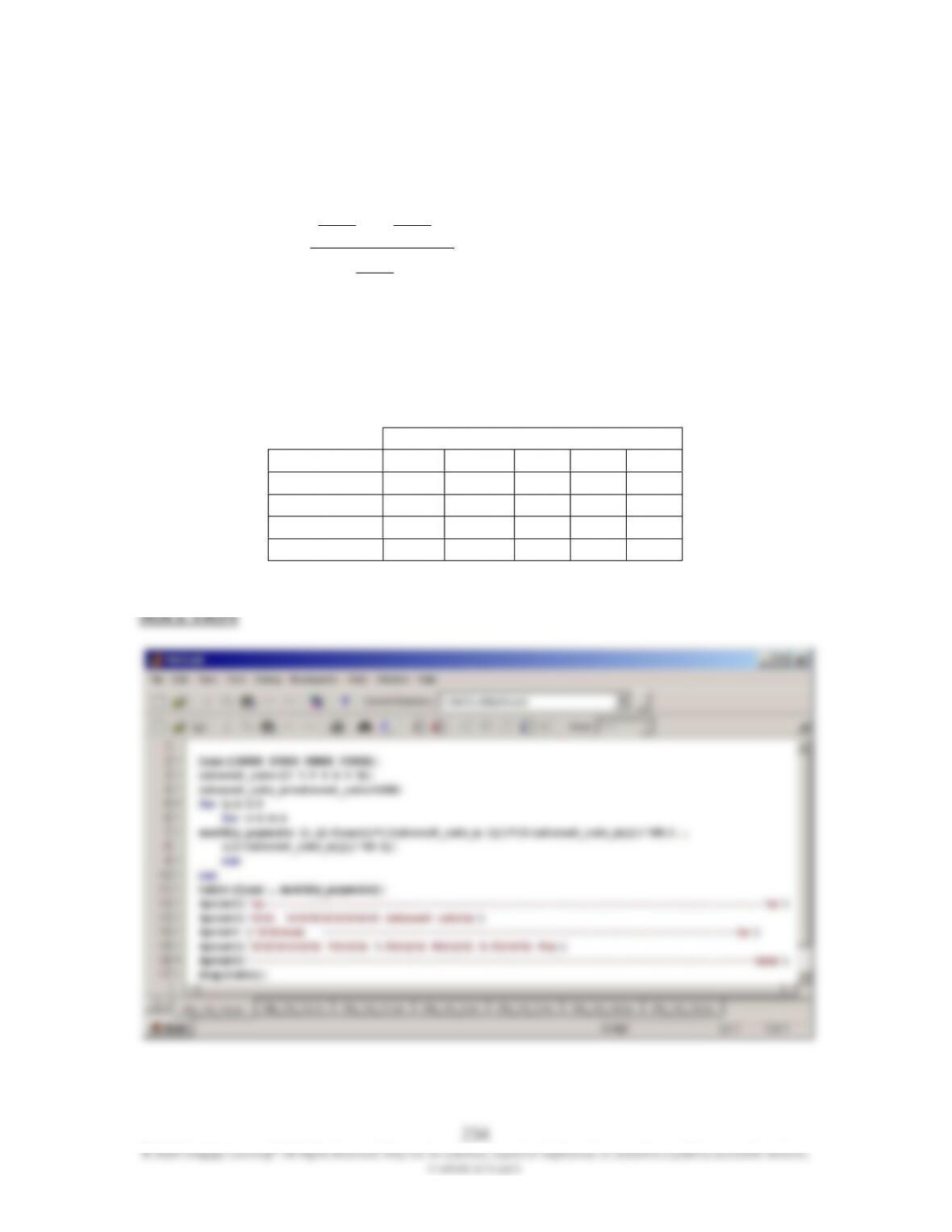
15.13 A person by the name of Huebscher developed a relationship between the
equivalent size of round ducts and the rectangular ducts according to:
25.0
625.0
)(
)(
3.1 ba
ab
D
where
D = diameter of equivalent circular duct (mm)
a = dimension of one side of the rectangular duct (mm)
b = dimension of the other side of the rectangular duct (mm)
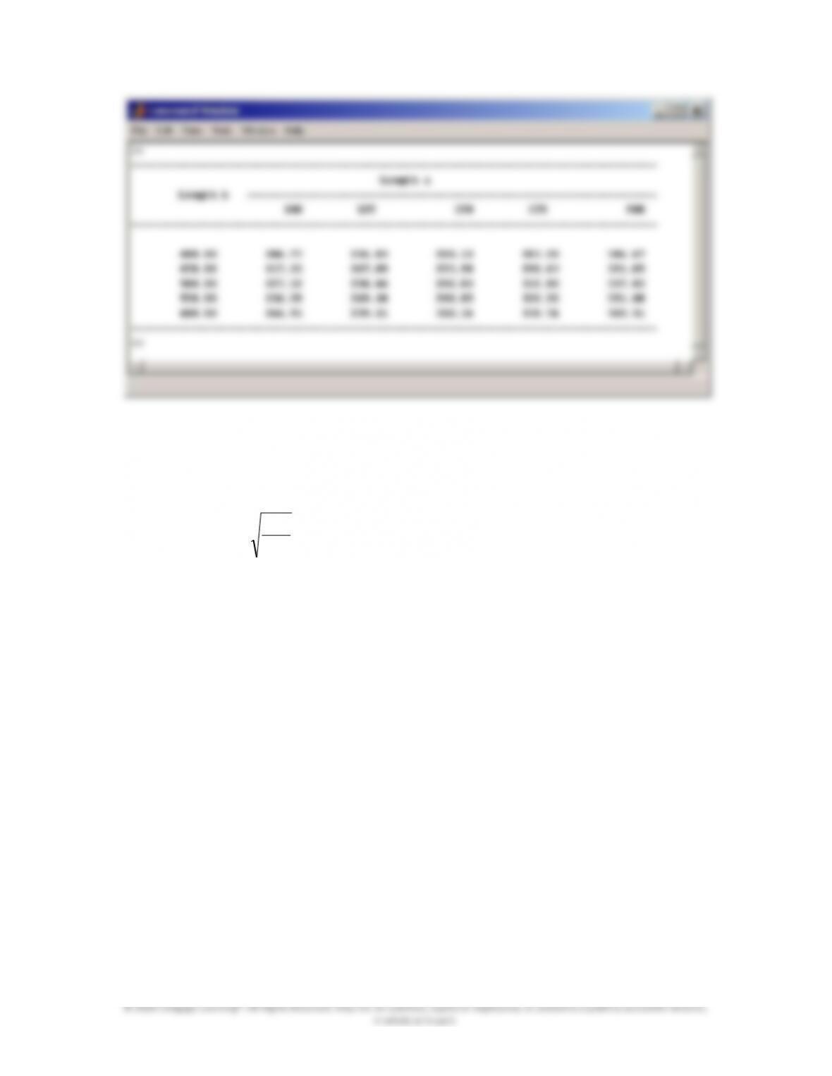
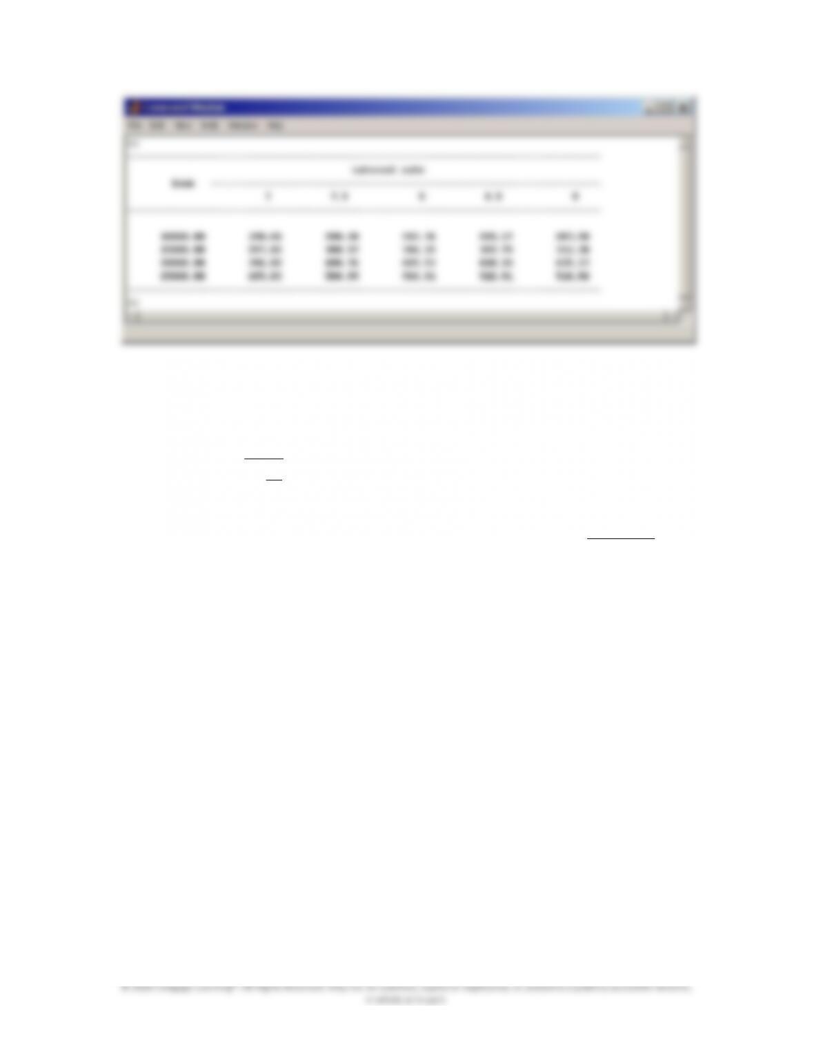
Using MATLAB, create a table that shows the relationship between the circular
and the rectangular duct, similar to the one shown in the accompanying table.
Length of One Side of
Rectangular Duct (length
a
)
,
mm
L
ength b
100
125
150
175
200
400
450
500
550
600
231
© 2020 Cengage Learning®. All Rights Reserved. May not be scanned, copied or duplicated, or posted to a publicly accessible website,
in whole or in part.
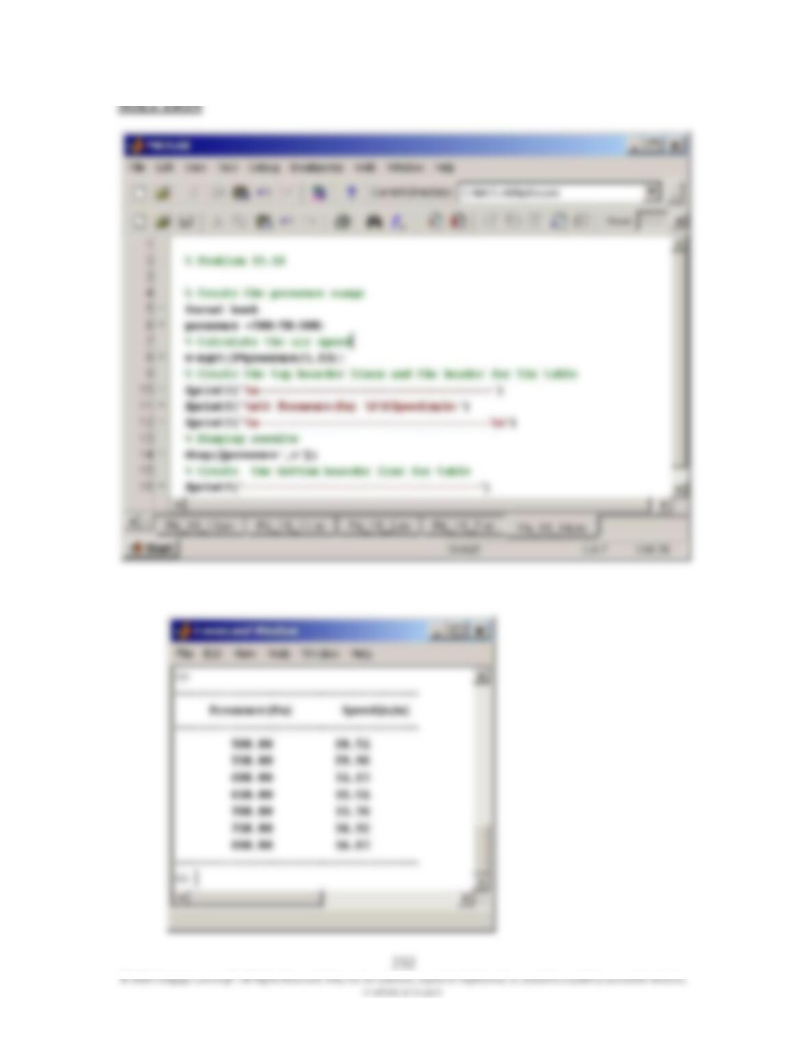
15.14 A Pitot tube is a device commonly used in a wind tunnel to measure the speed of
the air flowing over a model. The air speed is measured from the following
equation:
d
P
V2
where
V = air speed (m/s)
Pd = dynamic pressure (Pa)
= density of air (1.23 kg/m3)
Using MATLAB, create a table that shows the air speed for the range of dynamic
pressure of 500 Pa to 800 Pa. Use increments of 50 Pa.
232
© 2020 Cengage Learning®. All Rights Reserved. May not be scanned, copied or duplicated, or posted to a publicly accessible website,
in whole or in part.
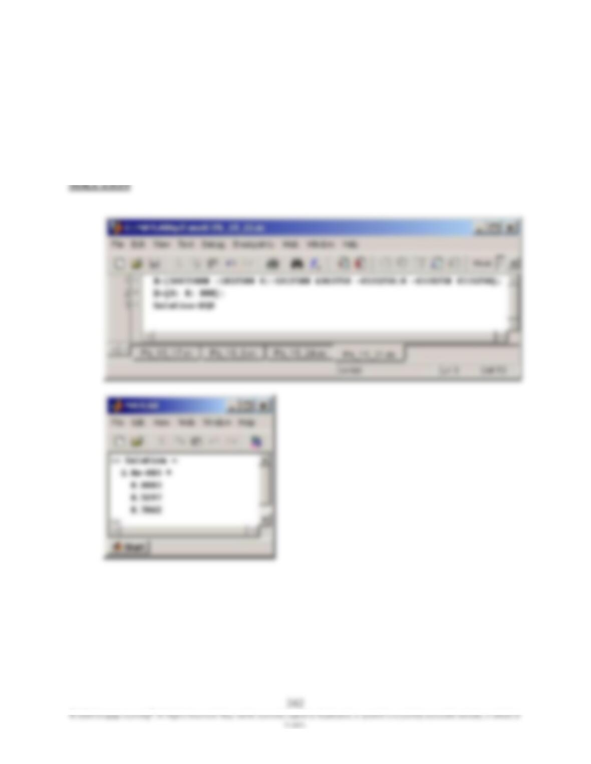
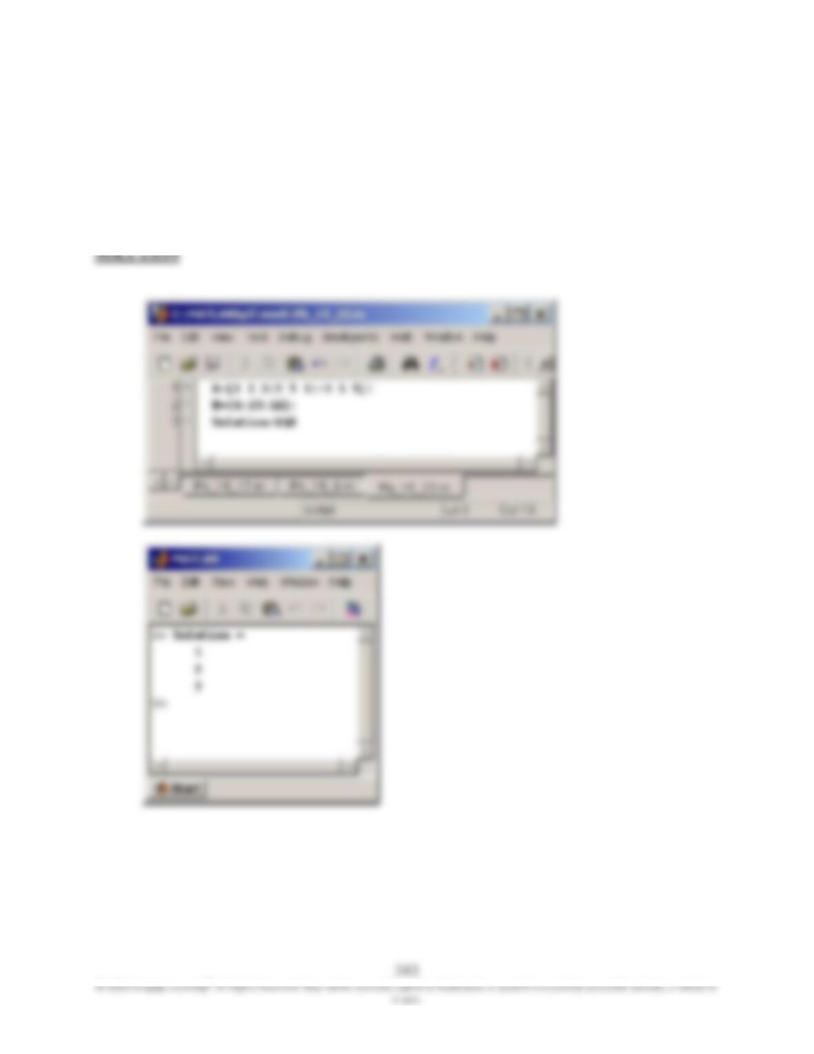
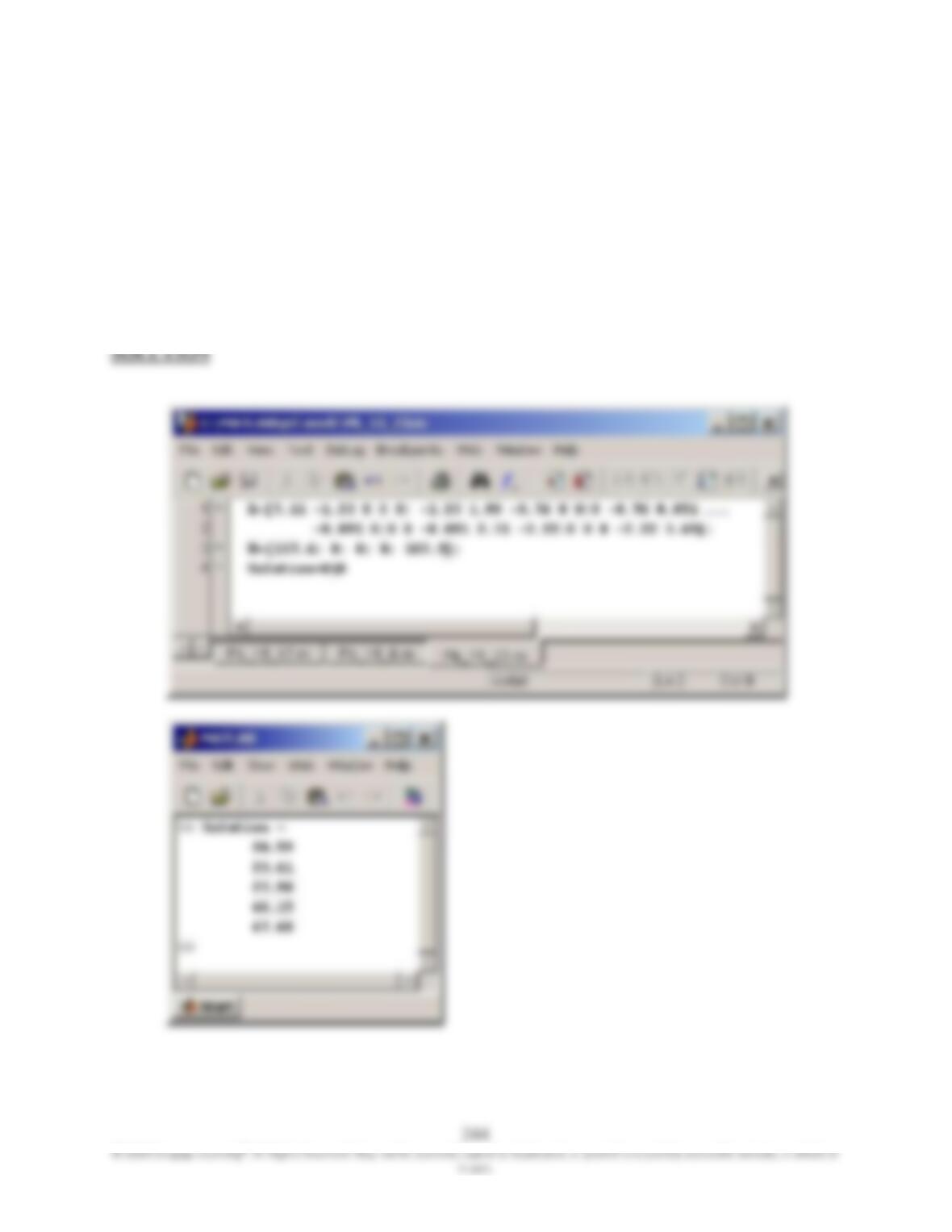
SOLUTION
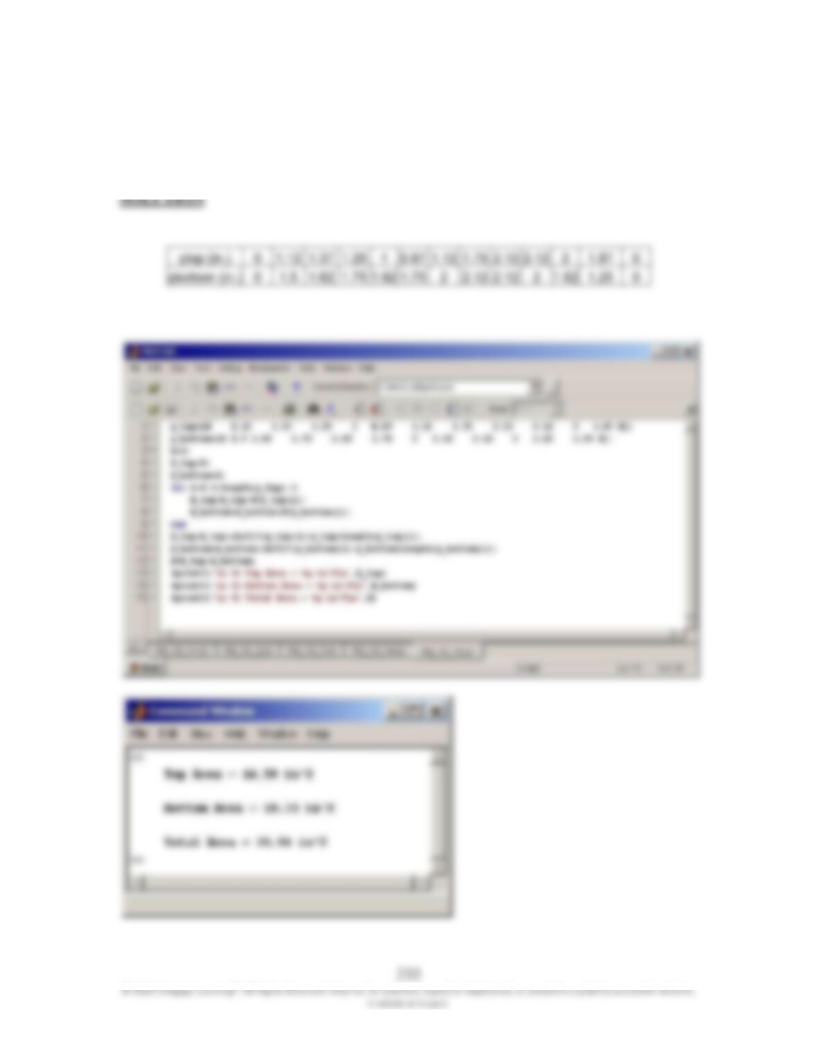
15.15 Use MATLAB to solve Example 7.1. Recall we applied the trapezoidal rule to
determine the area of the shape given. Create an Excel file with the given data,
and then import the file into MATLAB.
15.16 We will discuss engineering economics in Chapter 20. Using MATLAB, create a
table that can be used to lookup monthly payments on a car loan for a period of
five years. The monthly payments are calculated from:
1)
1200
1(
)
1200
1)(
1200
(
60
60
i
ii
PA
where
A = monthly payments in dollars
P = loan in dollars
i = interest rate, e.g. 7, 7.5, . . ., 9
Interest rate
Loan
7
7.5
8
8.5
9
10,000
15,000
20,000
25,000
235
© 2020 Cengage Learning®. All Rights Reserved. May not be scanned, copied or duplicated, or posted to a publicly accessible website,
in whole or in part.
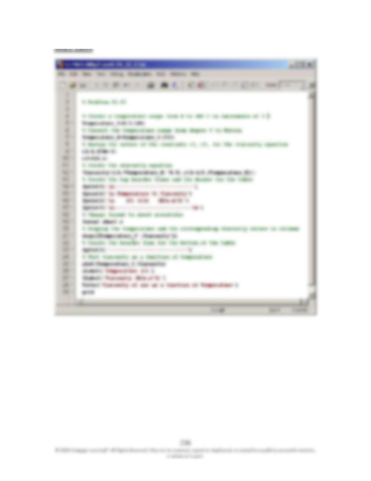
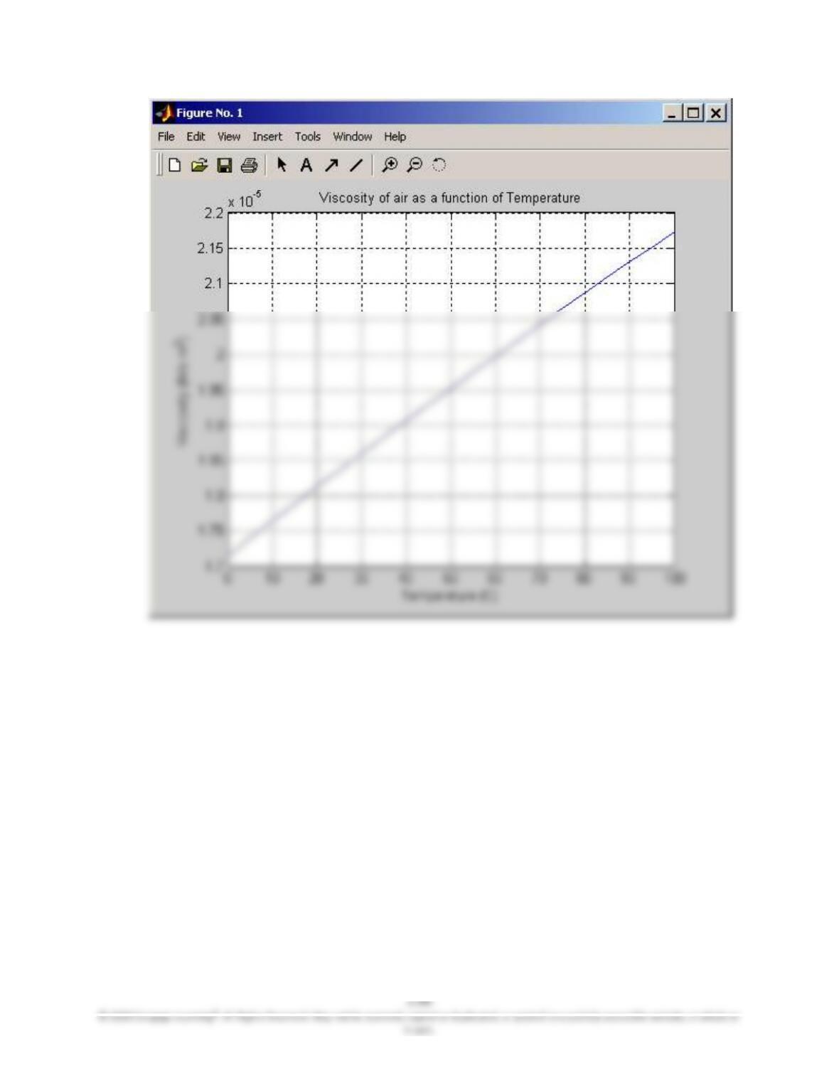
15.17 A person by the name of Sutterland has developed a correlation that can be used
to evaluate the viscosity of air as a function of temperature. It is given by:
T
c
Tc
2
5.0
1
1
where
= Viscosity (N/s·m2)
T = Temperature (K)
c1 = 1.458×10⁻⁶ ( 2/1
K
s
m
kg
)
c2 = 110.4 K
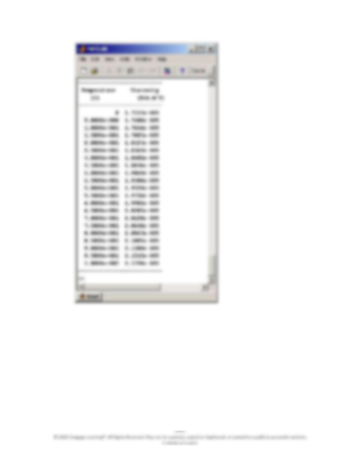
Create a table that shows the viscosity of air as a function of temperature in the
range of 0 C (273.15 K) to 100 C (373.15 K) in increments of 5 C. Also create
a graph showing the value of viscosity as a function of temperature.
236
© 2020 Cengage Learning®. All Rights Reserved. May not be scanned, copied or duplicated, or posted to a publicly accessible website,
in whole or in part.
SOLUTION
237
© 2020 Cengage Learning®. All Rights Reserved. May not be scanned, copied or duplicated, or posted to a publicly accessible website,
in whole or in part.
238
© 2020 Cengage Learning®. All Rights Reserved. May not be scanned, copied or duplicated, or posted to a publicly accessible website, in whole or
in part.
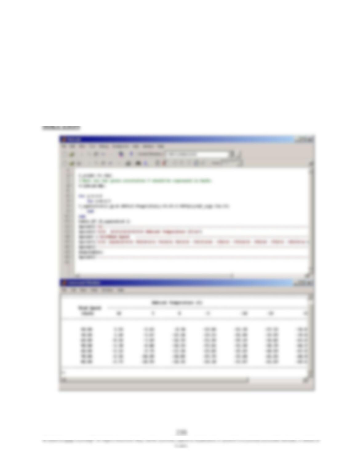
15.18 In Chapter 11, we explained the concept of wind chill factors. The old wind chill values
were determined empirically, and the common equivalent wind chill temperature Tequivalent
(C) was given by
33)33()28.045.102.5(045.0 5.0 aequivalent TVVT
Create a table that shows the wind-chill temperatures for the range of ambient air
temperature -30 C < Ta < 10 C and wind speed of 5 m/s < V < 20 m/s.
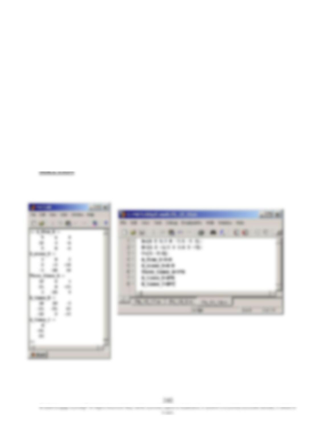
15.19 Given matrices:
351
707
124
A,
754
335
121
B, and
4
2
1
C, perform the following
operations using MATLAB.
a.
?
BA
b.
?
BA
c.
?3
A
d.
?
BA
e.
?
CA
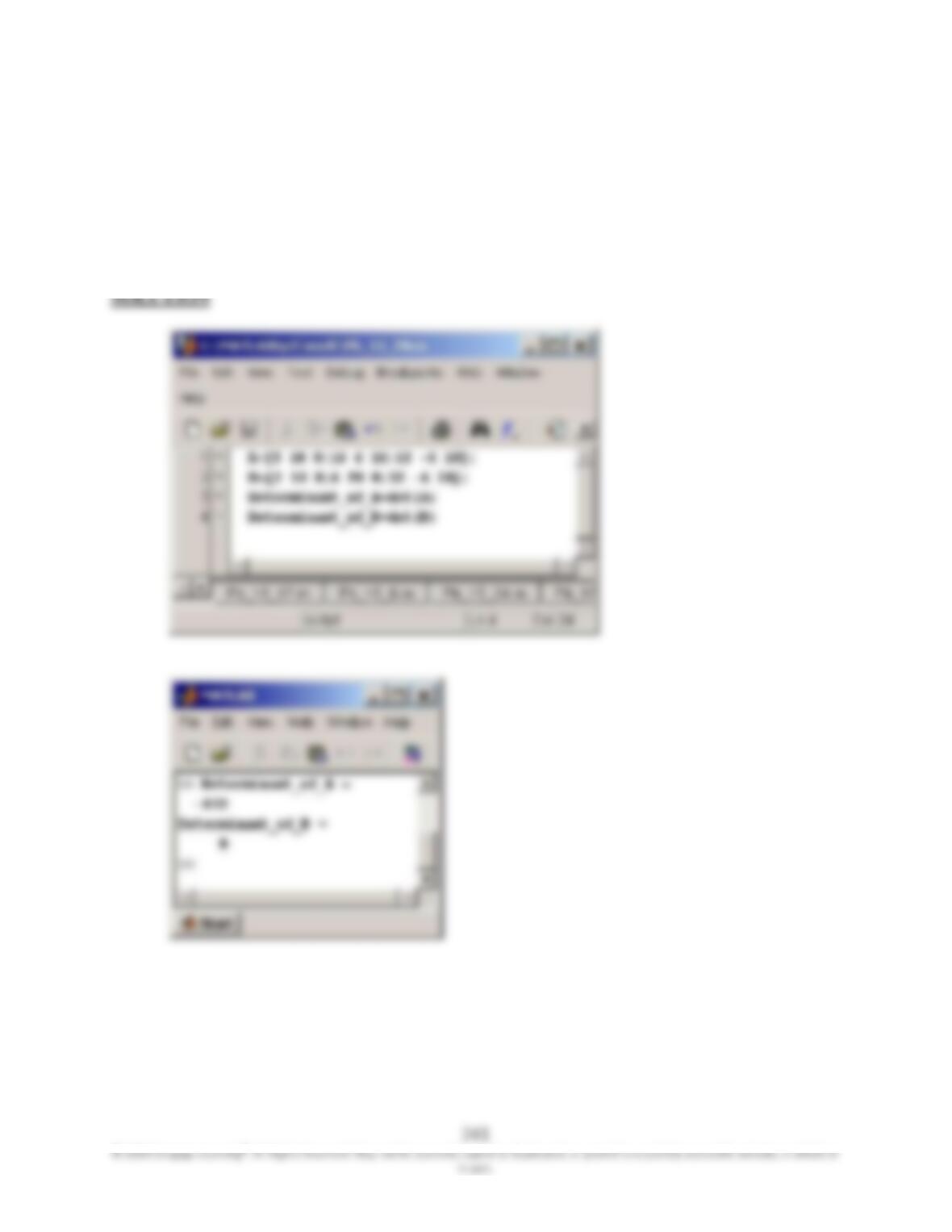
15.20 Given matrices:
18412
14616
0102
A , and
18412
0204
0102
B, calculate the determinant of [A] and [B]
using MATLAB.
15.21 Solve the following set of equations using MATLAB.
800
0
0
453125045312500
453125063437501812500
0181250010875000
3
2
1
u
u
u
15.22 Solve the following set of equations using MATLAB.
14
15
6
513
152
111
3
2
1
x
x
x
15.23 Solve the following set of equations using MATLAB.
9.102
0
0
0
6.117
69.322.2000
22.231.2091.000
0091.0851.076.00
0076.099.123.1
00023.111.7
5
4
3
2
1
T
T
T
T
T