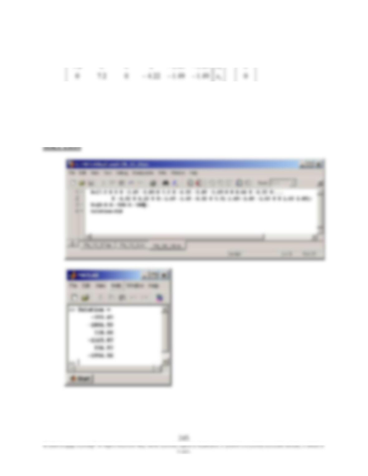
Civil Engineering Chapter 15 Solve The Following Set Equations Using Matlab Solution Cengage Learning Rights Reserved

15.24 Solve the following set of equations using MATLAB.



















































500

0

500

0

49.149.10049.149.1

49.171.5022.449.149.1

0022.4022.40

022.4044.800

6

5

4

3

2

x

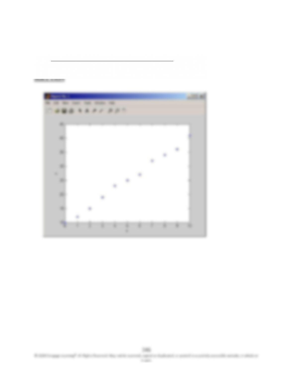
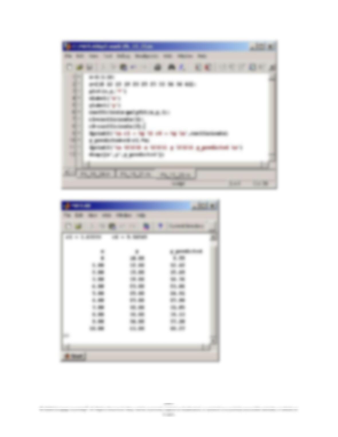
15.25 Find the equation that best fits the following set of data points. Compare the actual and

predicted values. Plot the data first.

x

0

1

2

3

4

5

6

7

8

9

10

y

10

12

15

19

23

25

27

32

34

36

41

247

in part.

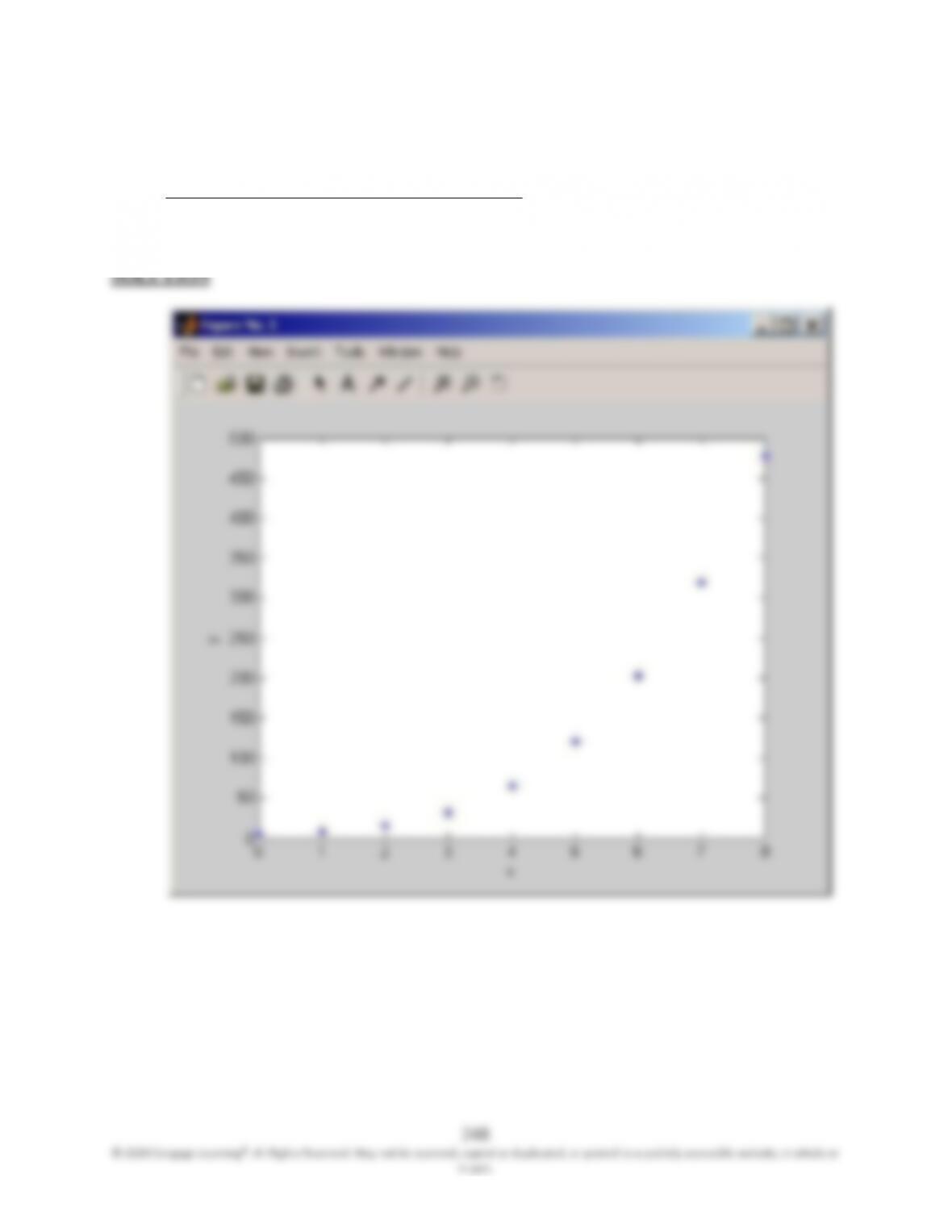
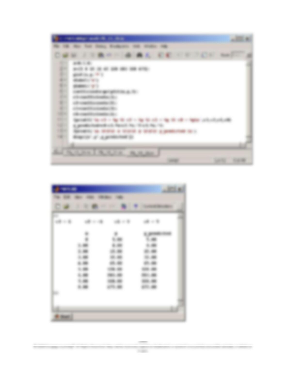
15.26 Find the equation that best fits the following set of data points. Compare the actual and

predicted values. Plot the data first.

x

0

1

2

3

4

5

6

7 8

y

5

8

15

32

65

120

203

320 477

249

in part.

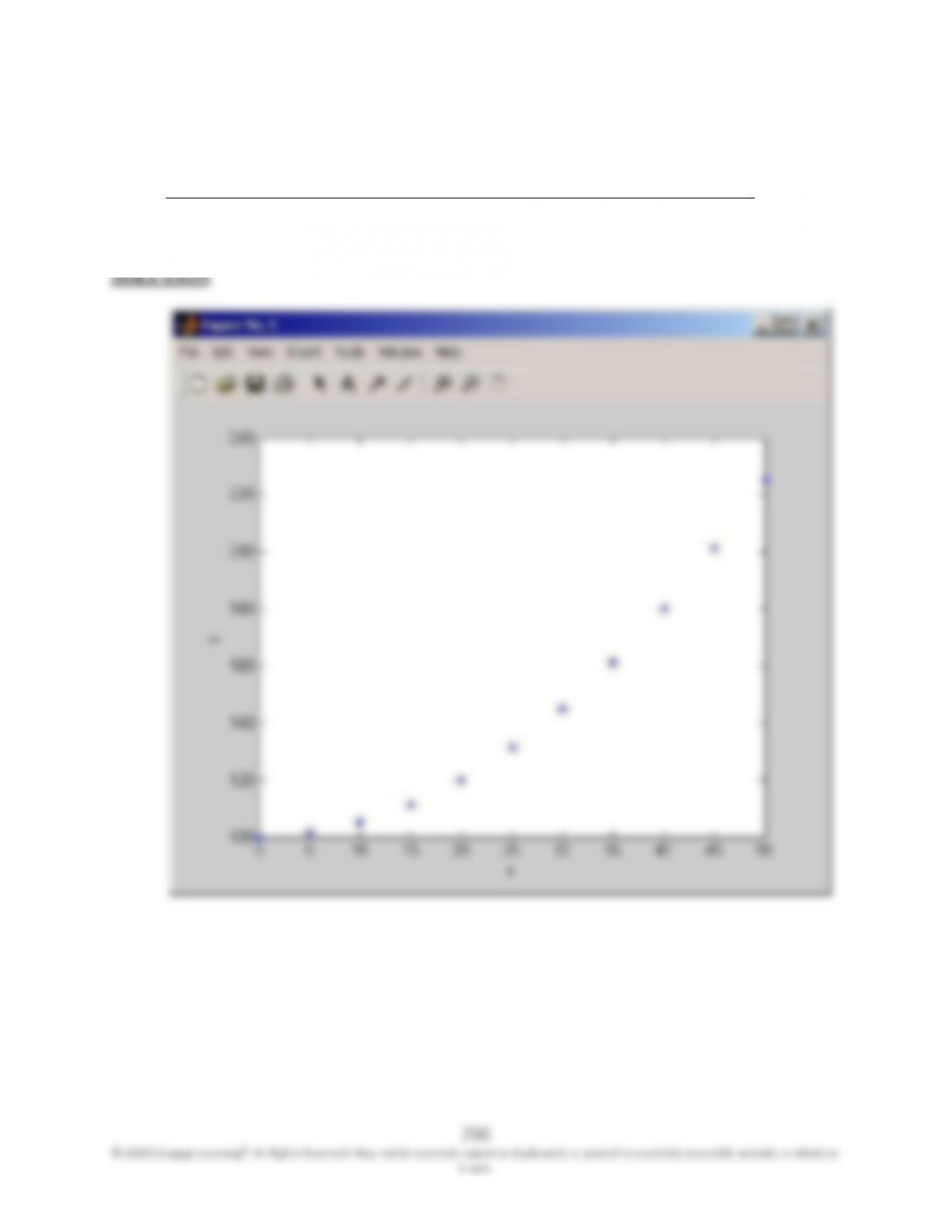
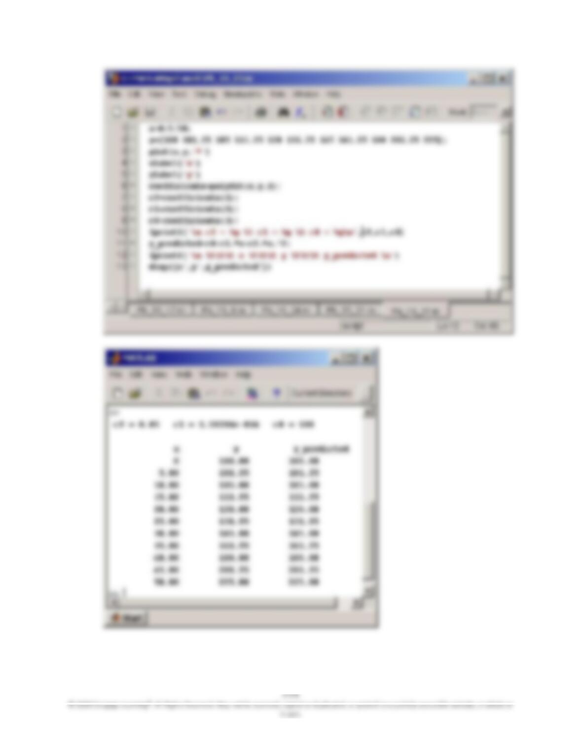
15.27 Find the equation that best fits the following set of data points. Compare the actual and

predicted values. Plot the data first.

x

0

5

10

15

20

25

30 35

40 45

50

y

100

101.25

105

111.25

120

131.25

145 161.25

180 201.25

225

251

in part.

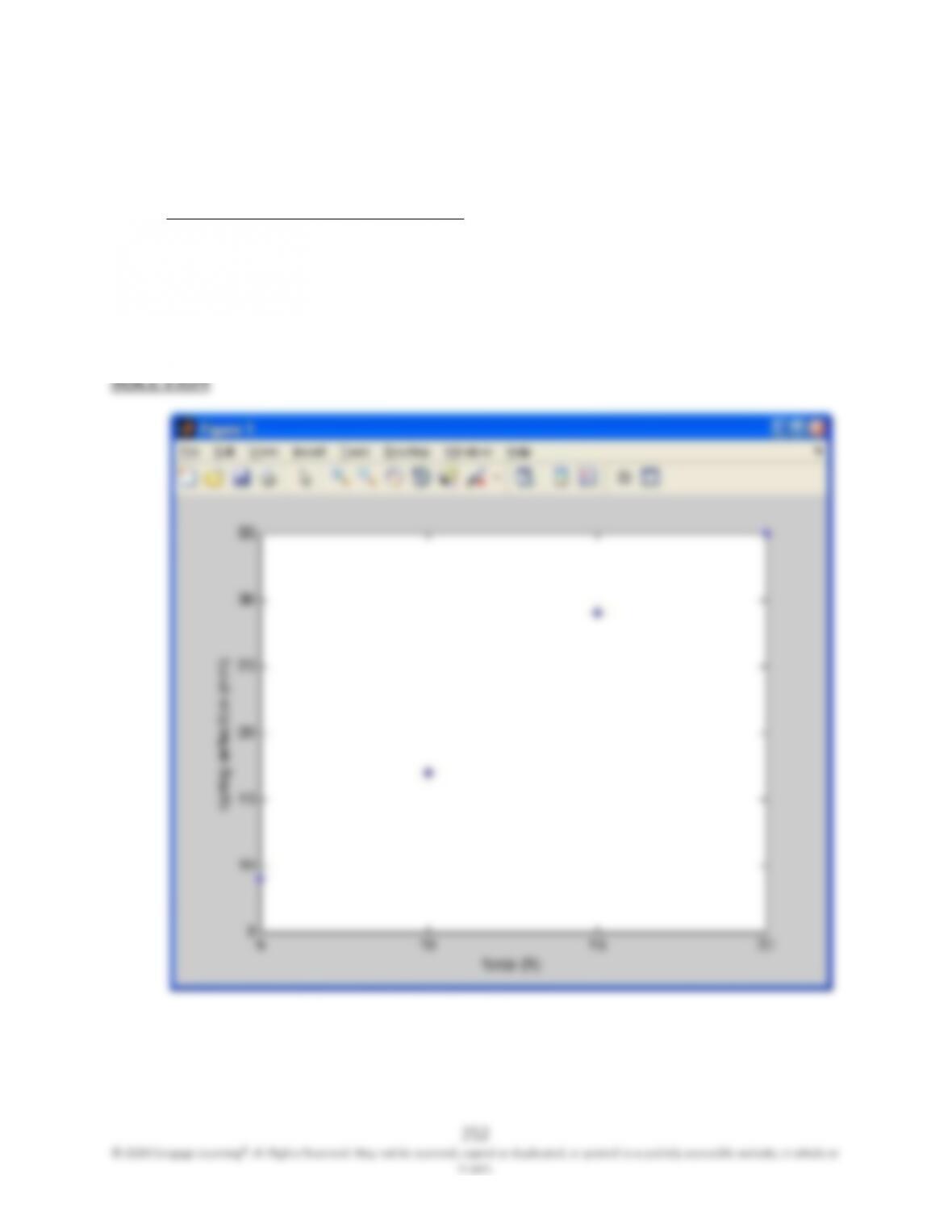
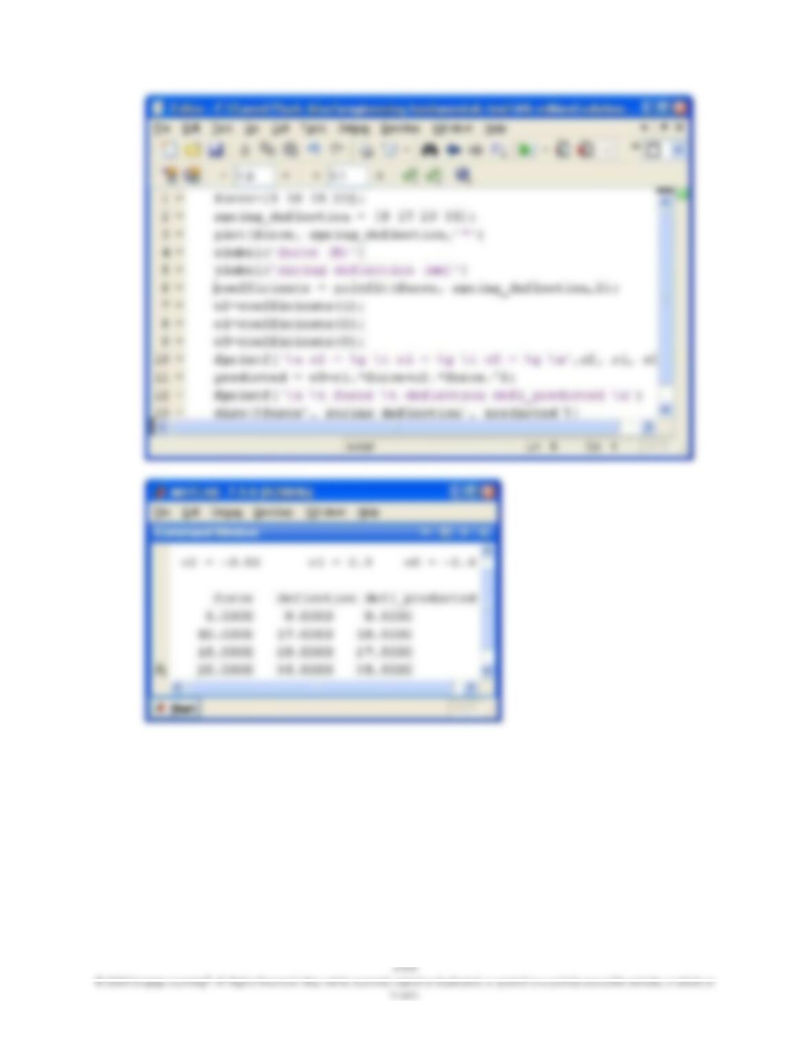
15.28 Find the equation that best fits the force-deflection data points given in the accompanying

table. Compare the actual and predicted force values. Plot the data first.

Force (N) Spring deflection

(mm)

5

9

10

17

15

29

20

35

253

in part.

254

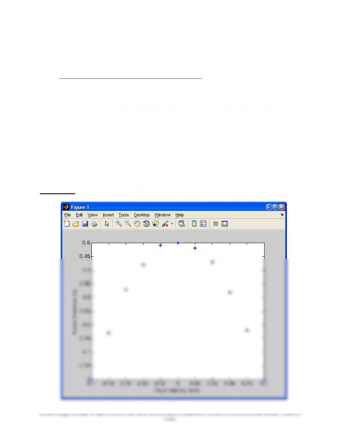
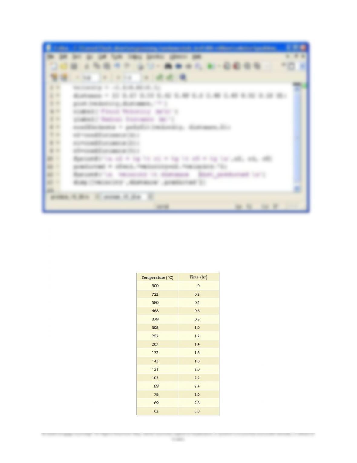
15.29 The data given in the accompanying table represents the velocity distribution inside a

pipe. Find the equation that best fits the fluid velocity-radial distance data given.

Compare the actual and predicted velocity values. Plot the data first.

Fluid Velocity (m/s)

Radial Distance (m)

–

0.1

0

–

0.08

0.17

–

0.06

0.33

–

0.04

0.42

–

0.02

0.49

0

0.5

0.02

0.48

0.04

0.43

0.06

0.32

0.08

0.18

0.1

0

SOLUTION

255

in part.

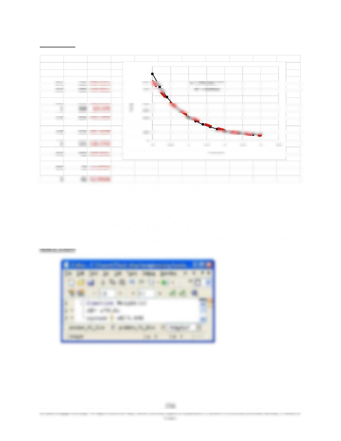
15.30 The data given in the accompanying table represents the cooling temperature of a plate

as a function of time during a material processing stage. Find the equation that best fits

the temperature-time data given. Compare the actual and predicted temperature

values. Plot the data first.

SOLUTION

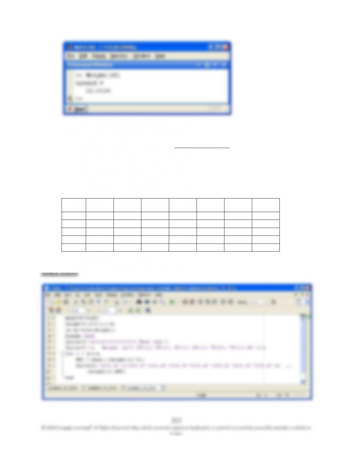
15.31 Write a function named Weight that when called in the command window will compute

the weight in pound force based on an input of mass in kilograms.

Actual Predicted

Time (hr) Temp ( C ) Temp ( C )

0 900 799.23

0.6 468 463.7978

1.4 207 224.494

1.8 143 156.1862

2.4 89 90.63575

2.8 69 63.05761

3 62 52.59646

0

100

200

300

600

900

1000

257

in part.

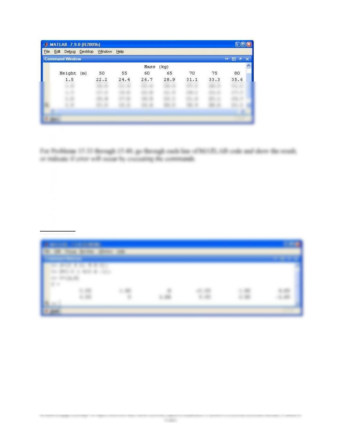
15.32 The Body Mass Index (BMI) is a way of determining obesity and whether someone is

overweight. It is computed from

 

2

)meterin (

)kgin (

height

mass

BMI . Write a program that will

create the table shown in accompanying figure. The BMI values in the range of 18.5 –

24.9, 25.0 – 29.9, and >30.0 are considered healthy, overweight, and obese, respectively.

Mass (kg)

Height

(m)

50

55

60

65

70

75

80

1.5

22.2 24.4 26.7 28.9 31.1 33.3 35.6

1.6

19.5 21.5 23.4 25.4 27.3 29.3 31.3

1.7

17.3 19.0 20.8 22.5 24.2 26.0 27.7

1.8

15.4 17.0 18.5 20.1 21.6 23.1 24.7

1.9

13.9 15.2 16.6 18.0 19.4 20.8 22.2

258

in part.

15.33 A =[3 1 0;4 0 1];

B =[-3 1 4;5 6 -1];

C=[A,B]

SOLUTION

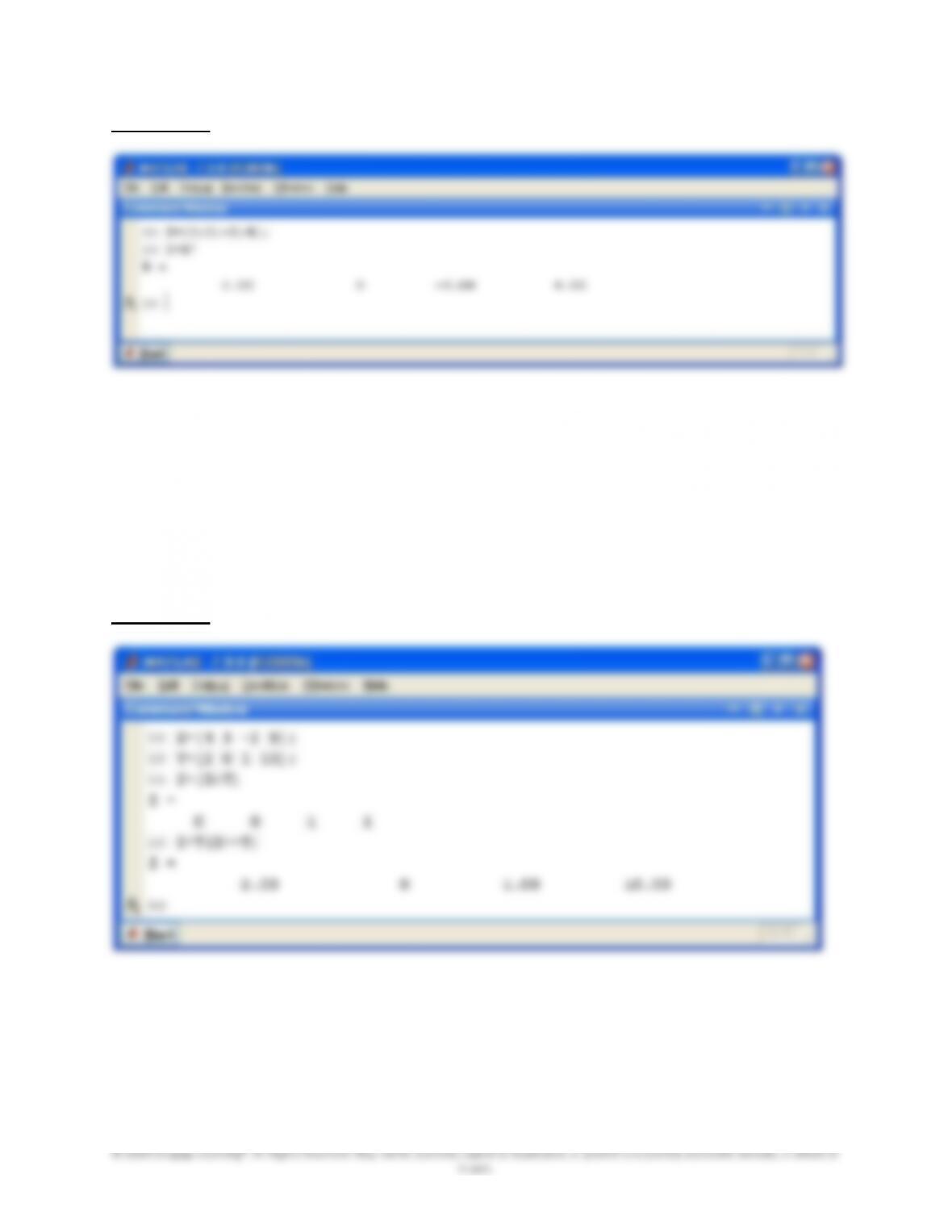
15.34 B=[1;0;-5;4];

D=B’

259

SOLUTION

15.35 X=[ 4 5 -2 8];

Y=[2 0 1 10];

Z=(X<Y)

Z=Y(X~ =Y)

SOLUTION

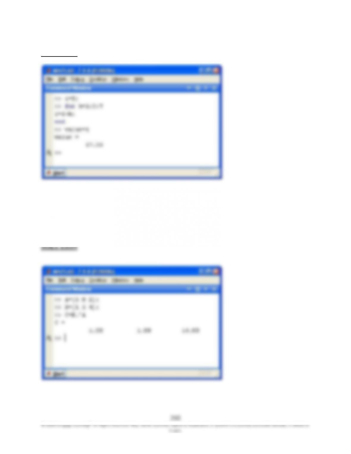
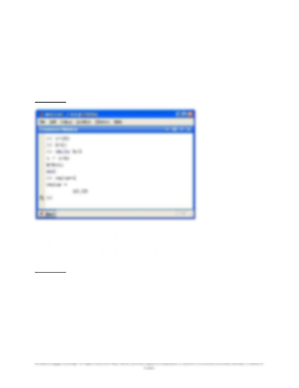
15.36 i=5

for k=1:3:7

i=i+k;

end

value=i

SOLUTION

15.37 A=[5 0 2];

B=[1 5 4];

C=B.^A

261

15.38 i=10;

k=2;

while k<4

i=i+k;

k=k+1;

end

value=i

SOLUTION

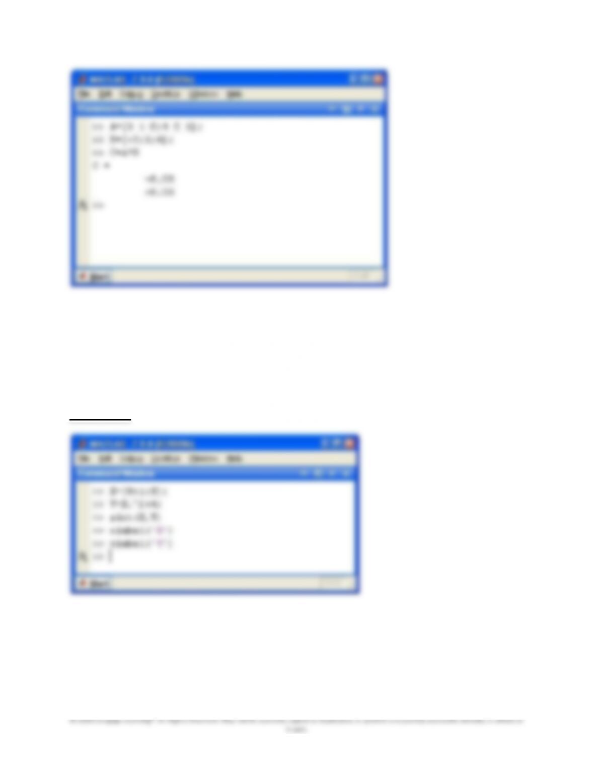
15.39 A =[3 1 0;4 0 1];

B =[-3; 1; 4];

C=A*B

SOLUTION

262

in part.

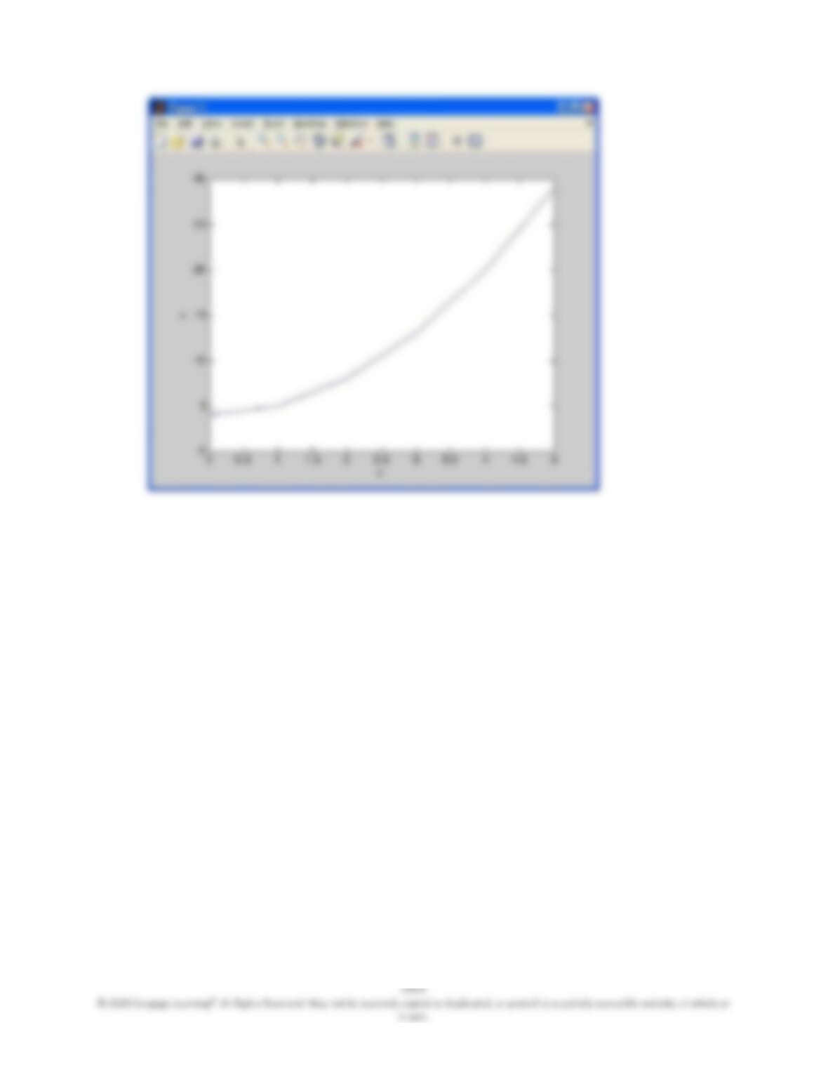
15.40 X = [0:1:5];

Y=X.^2+4;

plot(X,Y)

xlabel(‘X’)

ylabel(‘Y’)

SOLUTION

263

in part.