
205
Chapter 15: Computational Engineering Tools MATLAB
15.1 Using the MATLAB Help menu, discuss how the following functions are used.
Create a simple example and demonstrate the proper use of the function.
a. abs (x)
b. tic, toc
c. size (x)
d. fix (x)
e. floor (x)
f. ceil (x)
g. calendar
SOLUTION
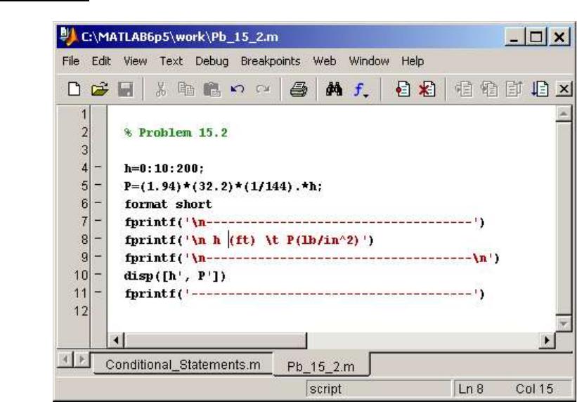
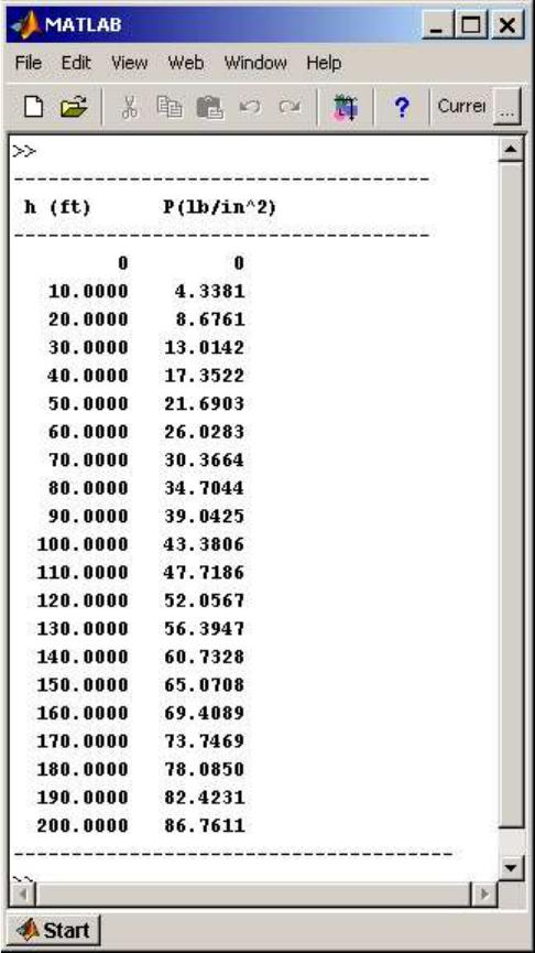
15.2 In Chapter 10, we discussed fluid pressure and the role of water towers in small
towns. Use MATLAB to create a table that shows the relationship between the
height of water above ground in the water tower and the water pressure in a pipe
line located at the base of the water tower. The relationship is given by:
ghP
where
P = water pressure at the base of the water tower (lb/ft2)
= density of water in slugs per cubic foot (= 1.94 slugs/ft3)
g = acceleration due to gravity (g = 32.2 ft/s2)
h = height of water above ground (ft)
Create a table that shows the water pressure in lb/in2 in a pipe located at the base
of the water tower as you vary the height of the water in increments of 10 ft. Also,
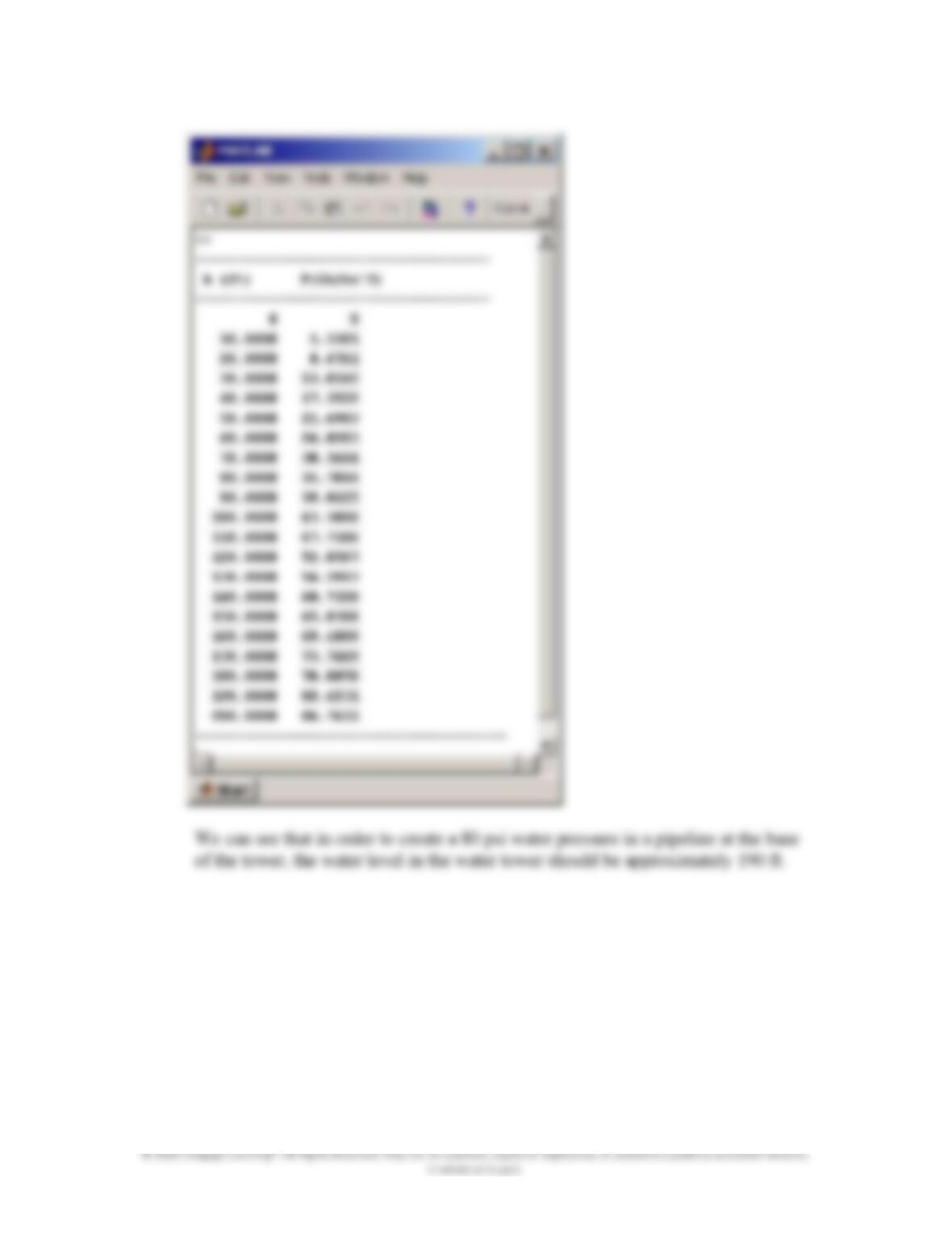
plot the water pressure (lb/in2) versus the height of water in feet. What should the
water level in the water tower be to create 80 psi of water pressure in a pipe at the
base of the water tower?
207
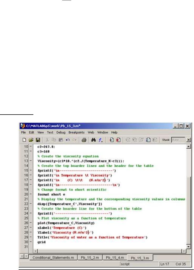
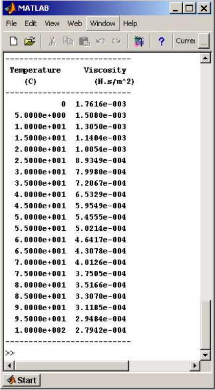
15.3 As we explained in Chapter 10, viscosity is a measure of how easily a fluid flows.
The viscosity of water can be determined from the following correlation
)(
1
3
2
10 cT
c
c
where
viscosity (N·s/m2)
T temperature (K)
c1 2.414 x 10⁻⁵(N/s·m2)
c2 247.8 K
c3 140 K
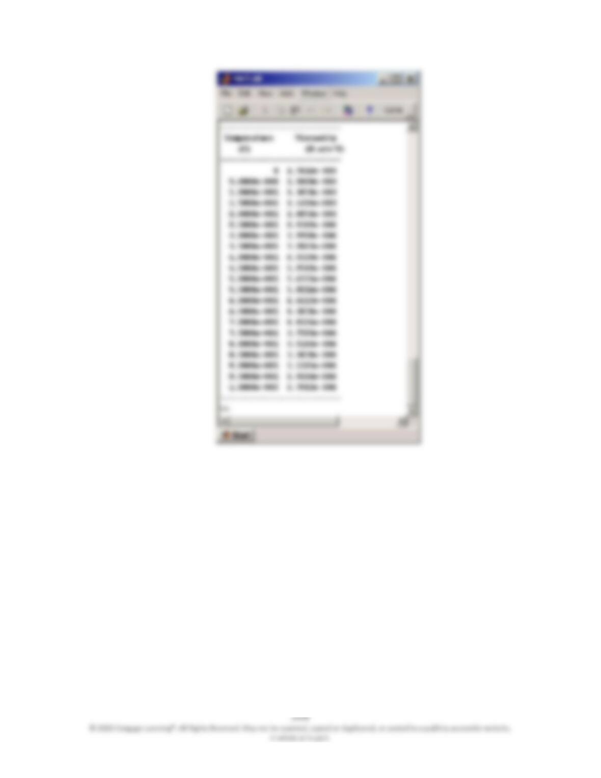
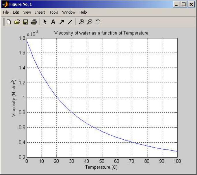
Using MATLAB, create a table that shows the viscosity of water as a function of
temperature in the range of 0 C (273.15 K) to 100 C (373.15 K) in increments
of 5 C. Also, create a graph showing the value of viscosity as a function of
temperature.
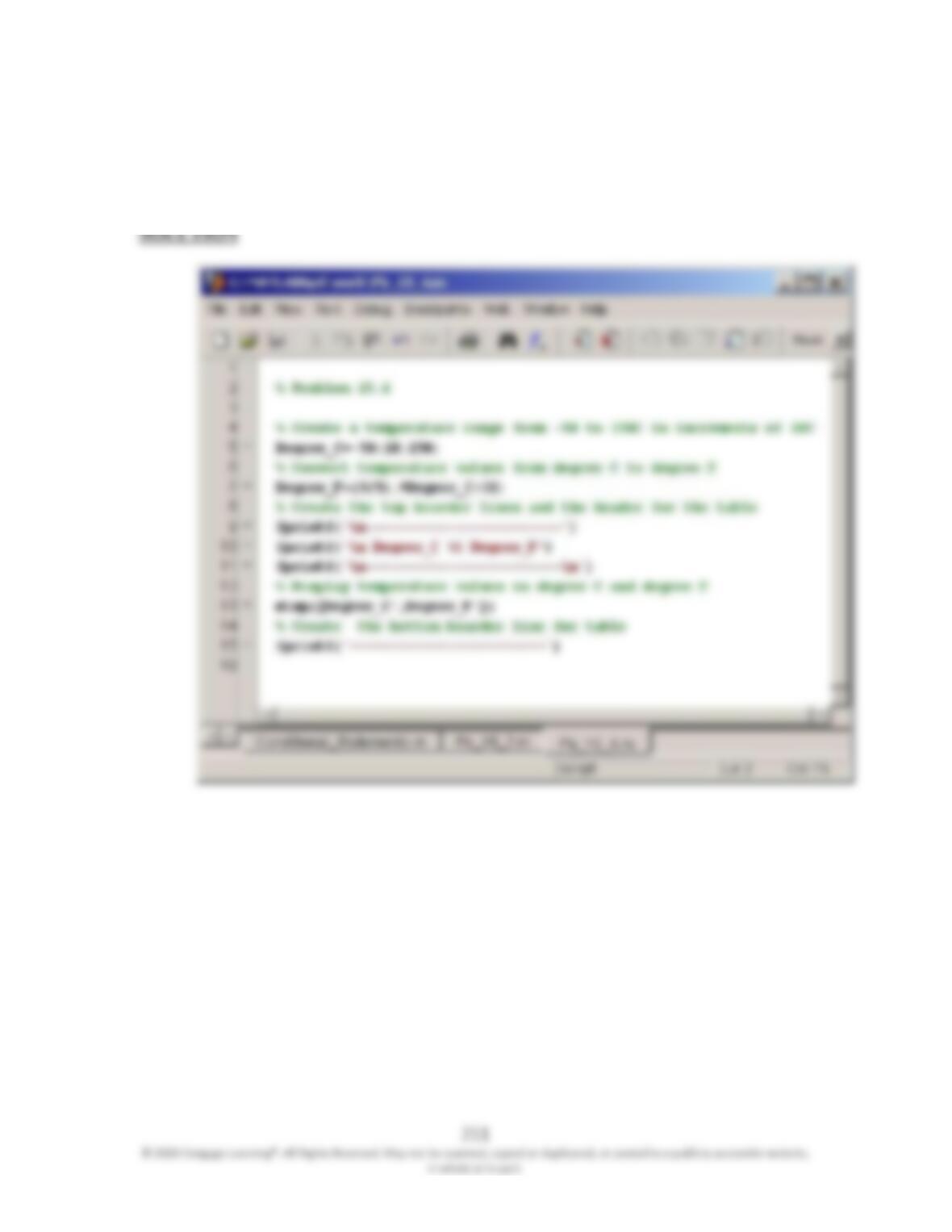
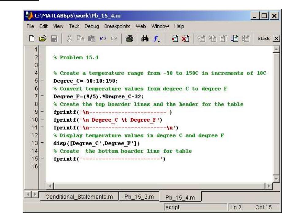
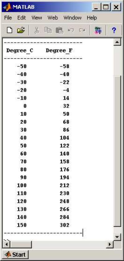
15.4 Using MATLAB, create a table that shows the relationship between the units of
temperature in degrees Celsius and Fahrenheit in the range of –50C to 150 C.
Use increments of 10C.
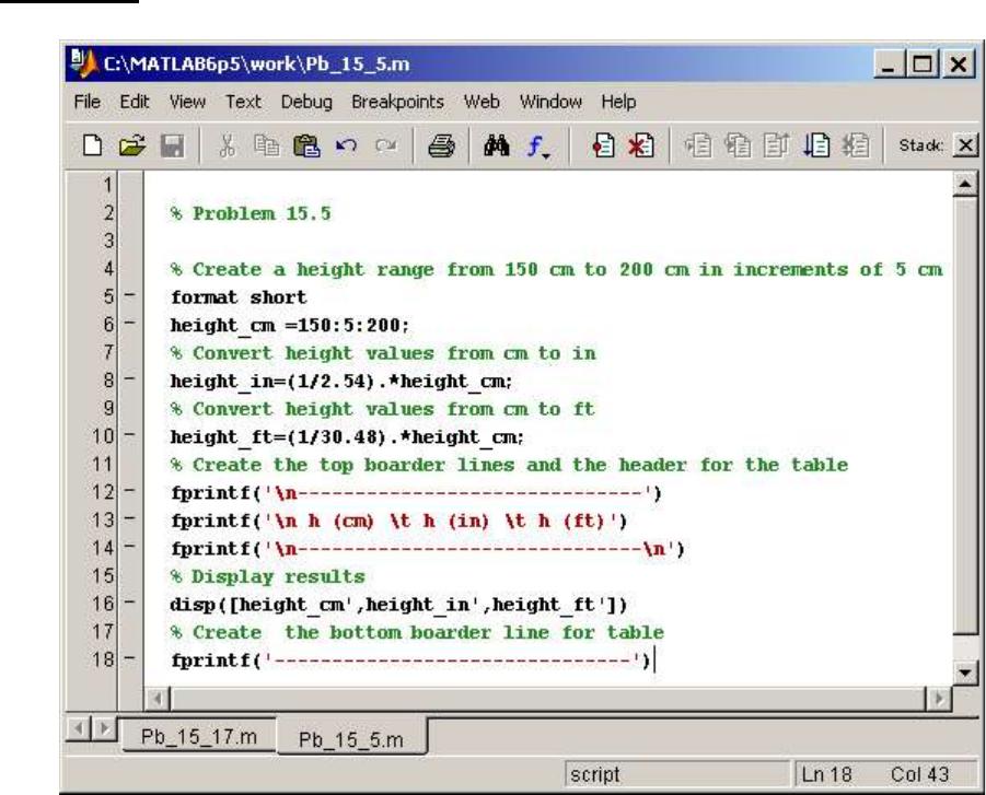
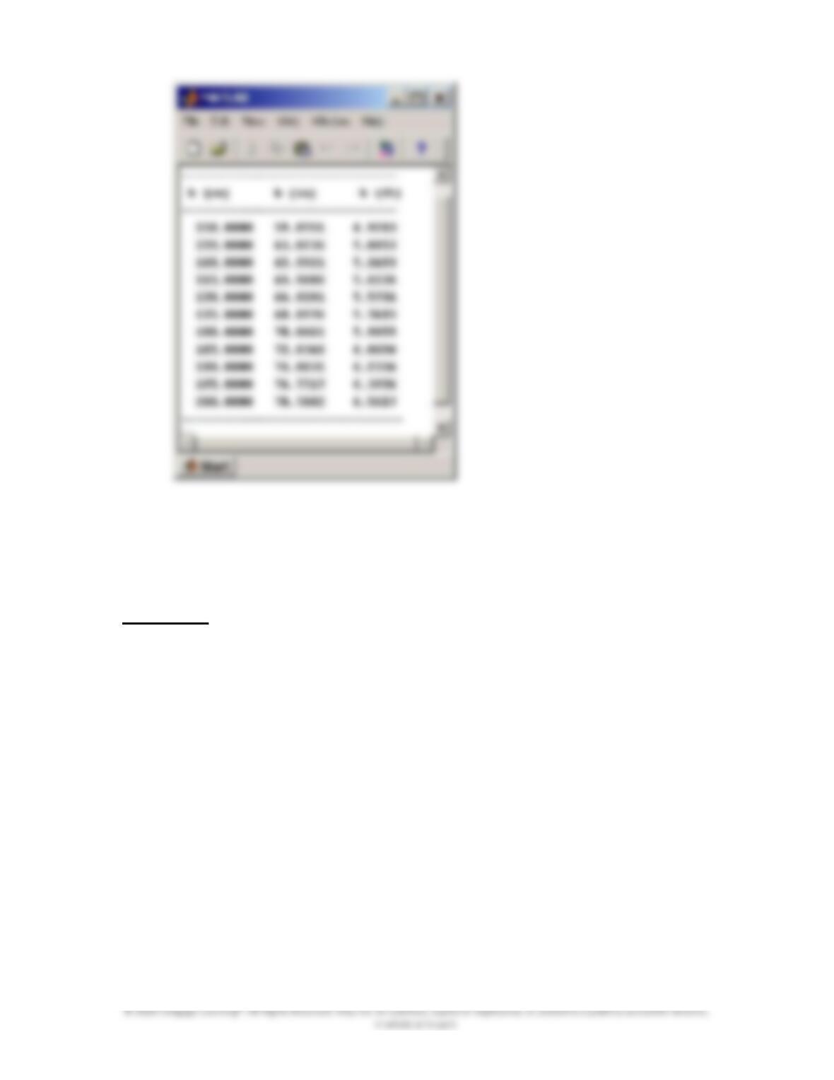
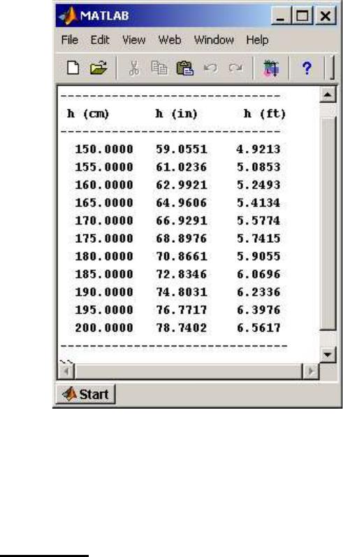
15.5 Using MATLAB, create a table that shows the relationship among the units of the
height of people in centimeters, inches, and feet in the range of 150 cm to 2 m.
Use increments of 5 cm.
214
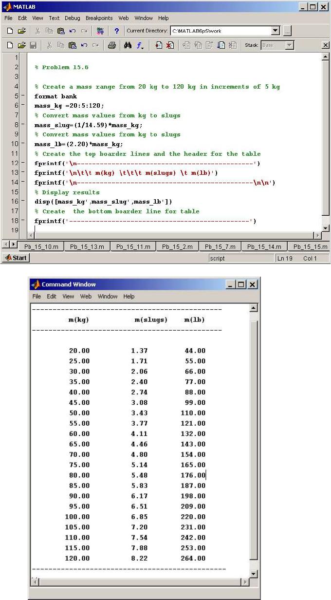
15.6 Using MATLAB, create a table that shows the relationship among the units of
mass to describe people’s mass in kilograms, slugs, and pound mass in the range
of 20 kg to 120 kg. Use increments of 5 kg.
SOLUTION
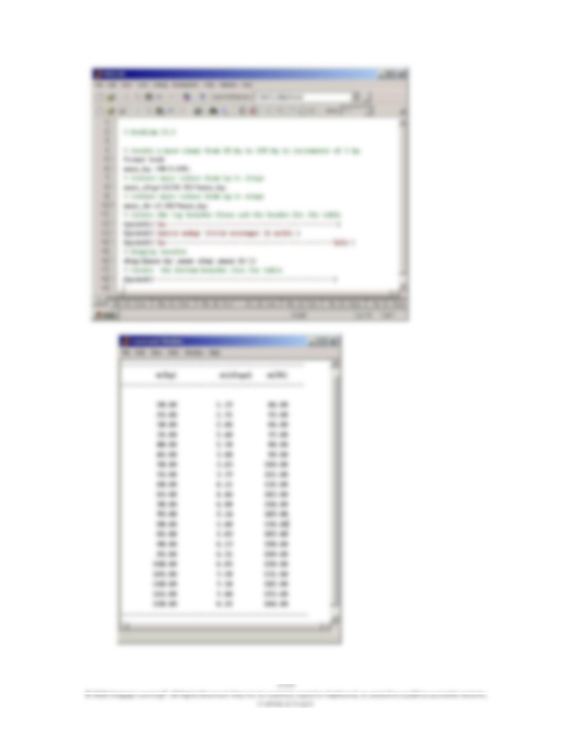
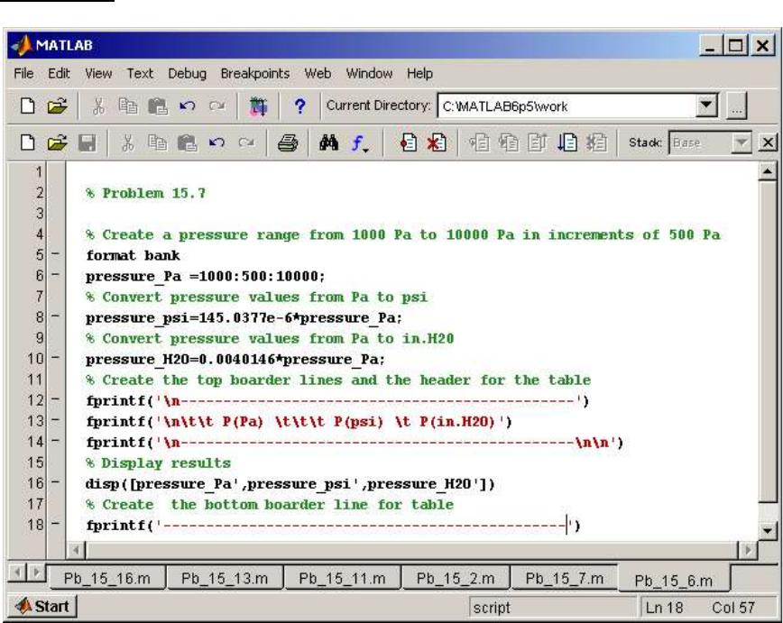
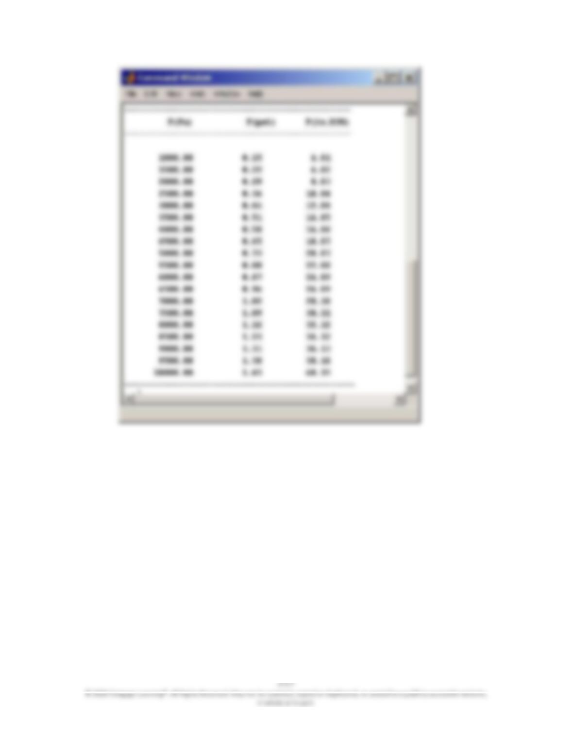
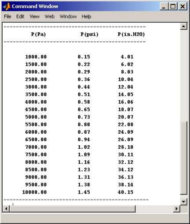
15.7 Using MATLAB, create a table that shows the relationship among the units of
pressure in Pa, psi, and inches of water in the range of 1000 Pa to 10,000 Pa. Use
increments of 500 Pa.
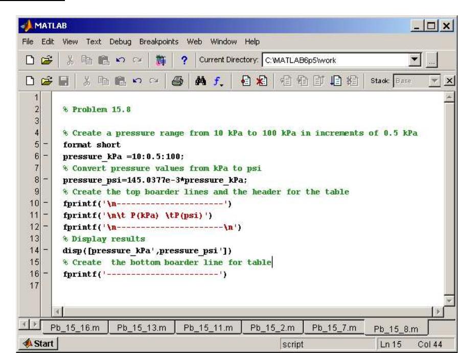
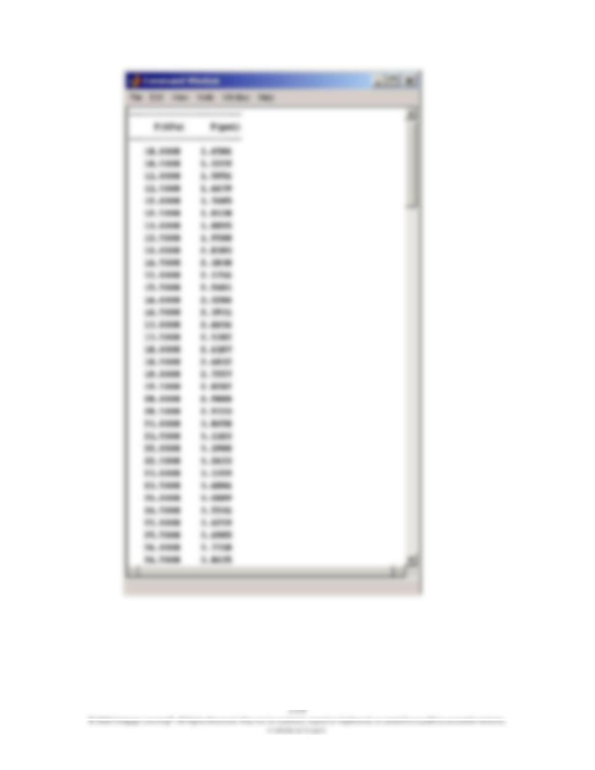
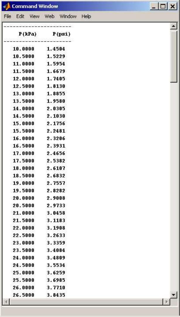
15.8 Using MATLAB, create a table that shows the relationship between the units of
pressure in Pa and psi in the range of 10 kPa to 100 kPa. Use increments of
0.5 kPa.
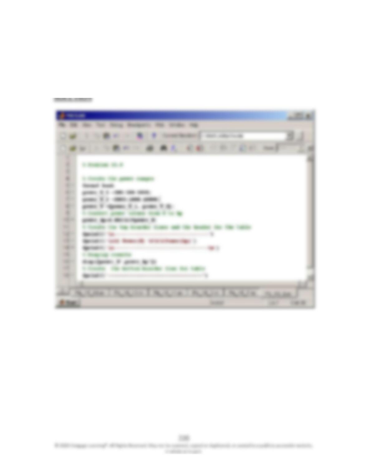
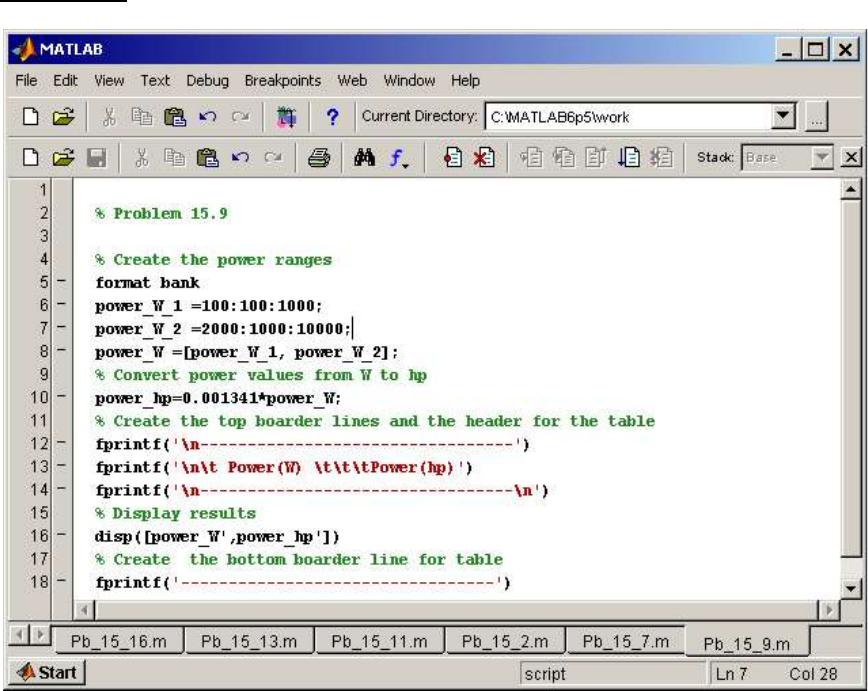
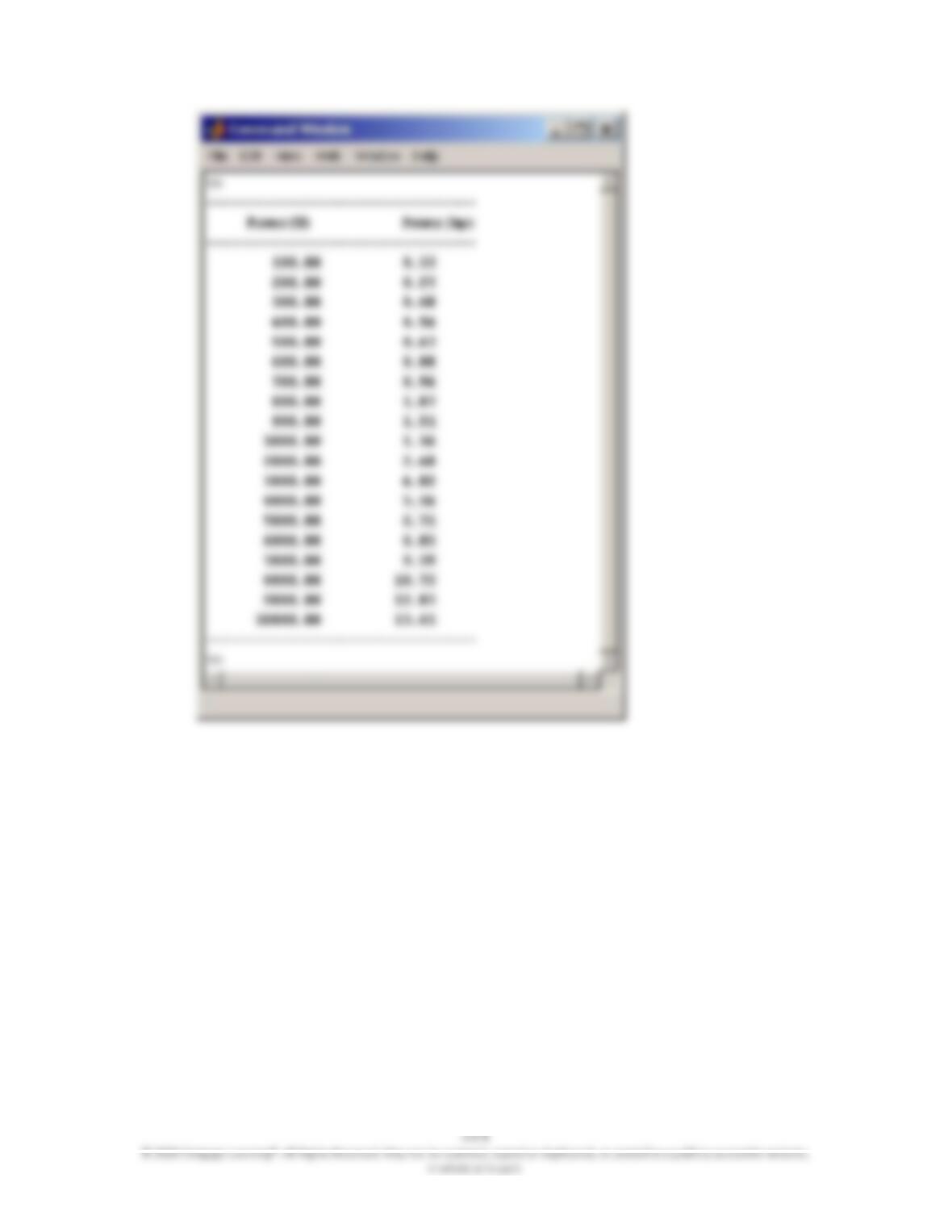
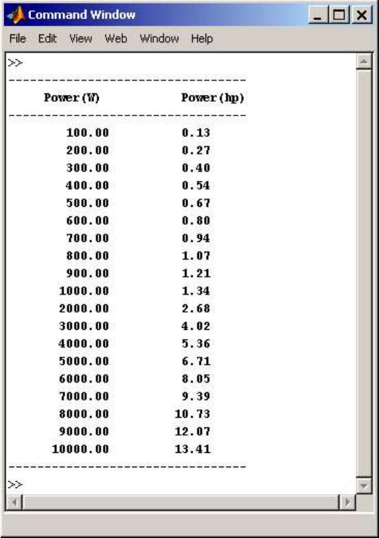
15.9 Using MATLAB, create a table that shows the relationship between the units of
power in watts and horsepower in the range of 100 W to 10,000 W. Use smaller
increments of 100 W up to 1000 W, and then use increments of 1000 W all the
way up to 10,000 W.


222
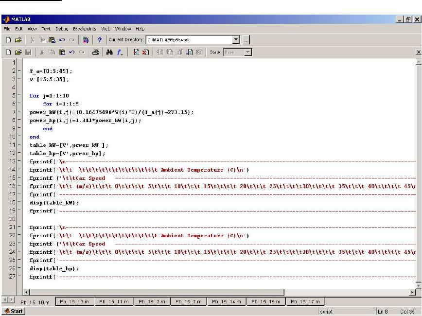
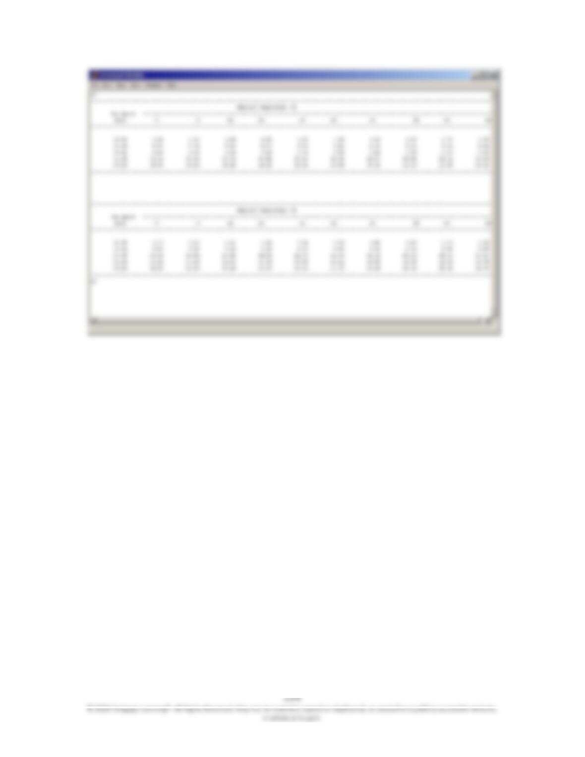
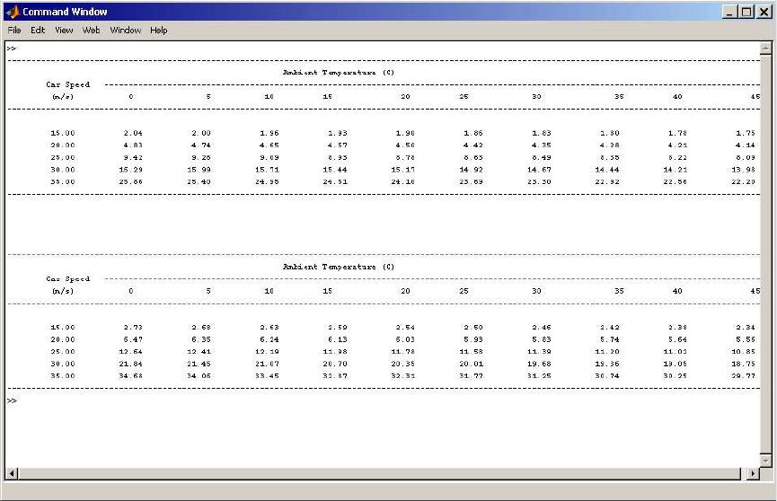
15.10 As we explained in earlier chapters, the air resistance to motion of a vehicle is
something important that engineers investigate. The drag force acting on a car is
determined experimentally by placing the car in a wind tunnel. The air speed
inside the tunnel is changed, and the drag force acting on the car is measured. For
a given car, the experimental data is generally represented by a single coefficient
that is called drag coefficient. It is defined by the following relationship:
AV
F
Cd
d
2
2
1
where
Cd = drag coefficient (unitless)
Fd = measured drag force (N or lb)
= air density (kg/m3 or slugs/ft3)
V = air speed inside the wind tunnel (m/s or ft/s)
A = frontal area of the car (m2 or ft2)
The frontal area A represents the frontal projection of the car’s area and could be
approximated simply by multiplying 0.85 times the width and the height of a
rectangle that outlines the front of a car. This is the area that you see when you
view the car from a direction normal to the front grill. The 0.85 factor is used to
adjust for rounded corners, open space below the bumper, and so on. To give you
some idea, typical drag coefficient values for sports cars are between 0.27 to 0.38
and for sedans are between 0.34 to 0.5.
The power requirement to overcome air resistance is computed by
VFP d
where
P = Power (Watts or ft.lb/sec)
1 horse power (hp) = 550 ft.lb/sec
and
1 horse power (hp) = 746 Watts
The purpose of this exercise is to see how the power requirement changes with the
car speed and the air temperature. Determine the power requirement to overcome
the air resistance for a car that has a listed drag coefficient of 0.4 and width of
74.4 inches and height of 57.4 inches. Vary the air speed in the range of 15 m/s <
V < 35 m/s, and change the air density range of 1.11 kg/m3 < <1.29 kg/m3. The
given air density range corresponds to 0C to 45C. You may use the ideal gas
law to relate the density of the air to its temperature. Present your findings in both
kilowatts and horsepower. Discuss your findings in terms of power consumption
as a function of speed and air temperature.